Class/Function Documentation
File I/O
open_image
-
open_image(file)¶ Locates & opens the specified hyperspectral image.
Arguments:
- file (str):
Name of the file to open.
Returns:
SpyFile object to access the file.
Raises:
IOError.
This function attempts to determine the associated file type and open the file. If the specified file is not found in the current directory, all directories listed in the
SPECTRAL_DATAenvironment variable will be searched until the file is found. If the file being opened is an ENVI file, the file argument should be the name of the header file.
ImageArray
-
class
ImageArray(data, spyfile)¶ ImageArray is an interface to an image loaded entirely into memory. ImageArray objects are returned by
spectral.SpyFile.load. This class inherits from both numpy.ndarray and Image, providing the interfaces of both classes.
SpyFile
-
class
SpyFile(params, metadata=None)¶ A base class for accessing spectral image files
-
__getitem__(args)¶ Subscripting operator that provides a numpy-like interface. Usage:
x = img[i, j]
x = img[i, j, k]
Arguments:
i, j, k (int or
sliceobject)Integer subscript indices or slice objects.
The subscript operator emulates the
numpy.ndarraysubscript operator, except data are read from the corresponding image file instead of an array object in memory. For frequent access or when accessing a large fraction of the image data, consider callingspectral.SpyFile.loadto load the data into anspectral.image.ImageArrayobject and using its subscript operator instead.Examples:
Read the pixel at the 30th row and 51st column of the image:
pixel = img[29, 50]
Read the 10th band:
band = img[:, :, 9]
Read the first 30 bands for a square sub-region of the image:
region = img[50:100, 50:100, :30]
-
__str__()¶ Prints basic parameters of the associated file.
-
load(**kwargs)¶ Loads entire image into memory in a
spectral.image.ImageArray.Keyword Arguments:
dtype (numpy.dtype):
An optional dtype to which the loaded array should be cast.
scale (bool, default True):
Specifies whether any applicable scale factor should be applied to the data after loading.
spectral.image.ImageArrayis derived from bothspectral.image.Imageandnumpy.ndarrayso it supports the fullnumpy.ndarrayinterface. The returns object will have shape (M,N,B), where M, N, and B are the numbers of rows, columns, and bands in the image.
-
SpyFile Subclasses
SpyFile is an abstract base class. Subclasses of SpyFile
(BipFile, BilFile,
BsqFile) all implement a common set of additional
methods. BipFile is shown here but the other two are similar.
-
class
BipFile(params, metadata=None)¶ A class to interface image files stored with bands interleaved by pixel.
-
open_memmap(**kwargs)¶ Returns a new numpy.memmap object for image file data access.
Keyword Arguments:
interleave (str, default ‘bip’):
Specifies the shape/interleave of the returned object. Must be one of [‘bip’, ‘bil’, ‘bsq’, ‘source’]. If not specified, the memmap will be returned as ‘bip’. If the interleave is ‘source’, the interleave of the memmap will be the same as the source data file. If the number of rows, columns, and bands in the file are R, C, and B, the shape of the returned memmap array will be as follows:
interleave
array shape
‘bip’
(R, C, B)
‘bil’
(R, B, C)
‘bsq’
(B, R, C)
writable (bool, default False):
If writable is True, modifying values in the returned memmap will result in corresponding modification to the image data file.
-
read_band(band, use_memmap=True)¶ Reads a single band from the image.
Arguments:
band (int):
Index of band to read.
use_memmap (bool, default True):
Specifies whether the file’s memmap interface should be used to read the data. Setting this arg to True only has an effect if a memmap is being used (i.e., if img.using_memmap is True).
Returns:
numpy.ndarrayAn MxN array of values for the specified band.
-
read_bands(bands, use_memmap=True)¶ Reads multiple bands from the image.
Arguments:
bands (list of ints):
Indices of bands to read.
use_memmap (bool, default True):
Specifies whether the file’s memmap interface should be used to read the data. Setting this arg to True only has an effect if a memmap is being used (i.e., if img.using_memmap is True).
Returns:
numpy.ndarrayAn MxNxL array of values for the specified bands. M and N are the number of rows & columns in the image and L equals len(bands).
-
read_pixel(row, col, use_memmap=True)¶ Reads the pixel at position (row,col) from the file.
Arguments:
row, col (int):
Indices of the row & column for the pixel
use_memmap (bool, default True):
Specifies whether the file’s memmap interface should be used to read the data. Setting this arg to True only has an effect if a memmap is being used (i.e., if img.using_memmap is True).
Returns:
numpy.ndarrayA length-B array, where B is the number of image bands.
-
read_subimage(rows, cols, bands=None, use_memmap=False)¶ Reads arbitrary rows, columns, and bands from the image.
Arguments:
rows (list of ints):
Indices of rows to read.
cols (list of ints):
Indices of columns to read.
bands (list of ints):
Optional list of bands to read. If not specified, all bands are read.
use_memmap (bool, default False):
Specifies whether the file’s memmap interface should be used to read the data. Setting this arg to True only has an effect if a memmap is being used (i.e., if img.using_memmap is True).
Returns:
numpy.ndarrayAn MxNxL array, where M = len(rows), N = len(cols), and L = len(bands) (or # of image bands if bands == None).
-
read_subregion(row_bounds, col_bounds, bands=None, use_memmap=True)¶ Reads a contiguous rectangular sub-region from the image.
Arguments:
row_bounds (2-tuple of ints):
(a, b) -> Rows a through b-1 will be read.
col_bounds (2-tuple of ints):
(a, b) -> Columnss a through b-1 will be read.
bands (list of ints):
Optional list of bands to read. If not specified, all bands are read.
use_memmap (bool, default True):
Specifies whether the file’s memmap interface should be used to read the data. Setting this arg to True only has an effect if a memmap is being used (i.e., if img.using_memmap is True).
Returns:
numpy.ndarrayAn MxNxL array.
-
SubImage
-
class
SubImage(image, row_range, col_range)¶ Represents a rectangular sub-region of a larger SpyFile object.
-
read_band(band)¶ Reads a single band from the image.
Arguments:
band (int):
Index of band to read.
Returns:
numpy.ndarrayAn MxN array of values for the specified band.
-
read_bands(bands)¶ Reads multiple bands from the image.
Arguments:
bands (list of ints):
Indices of bands to read.
Returns:
numpy.ndarrayAn MxNxL array of values for the specified bands. M and N are the number of rows & columns in the image and L equals len(bands).
-
read_pixel(row, col)¶ Reads the pixel at position (row,col) from the file.
Arguments:
row, col (int):
Indices of the row & column for the pixel
Returns:
numpy.ndarrayA length-B array, where B is the number of image bands.
-
read_subimage(rows, cols, bands=[])¶ Reads arbitrary rows, columns, and bands from the image.
Arguments:
rows (list of ints):
Indices of rows to read.
cols (list of ints):
Indices of columns to read.
bands (list of ints):
Optional list of bands to read. If not specified, all bands are read.
Returns:
numpy.ndarrayAn MxNxL array, where M = len(rows), N = len(cols), and L = len(bands) (or # of image bands if bands == None).
-
read_subregion(row_bounds, col_bounds, bands=None)¶ Reads a contiguous rectangular sub-region from the image.
Arguments:
row_bounds (2-tuple of ints):
(a, b) -> Rows a through b-1 will be read.
col_bounds (2-tuple of ints):
(a, b) -> Columnss a through b-1 will be read.
bands (list of ints):
Optional list of bands to read. If not specified, all bands are read.
Returns:
numpy.ndarrayAn MxNxL array.
-
File Formats
AVIRIS
Functions for handling AVIRIS image files.
-
open(file, band_file=None)¶ Returns a SpyFile object for an AVIRIS image file.
Arguments:
file (str):
Name of the AVIRIS data file.
band_file (str):
Optional name of the AVIRIS spectral calibration file.
Returns:
A SpyFile object for the image file.
Raises:
spectral.io.spyfile.InvalidFileError
-
read_aviris_bands(cal_filename)¶ Returns a BandInfo object for an AVIRIS spectral calibration file.
Arguments:
cal_filename (str):
Name of the AVIRIS spectral calibration file.
Returns:
A
spectral.BandInfoobject
ENVI
ENVI 1 is a popular commercial software package for processing
and analyzing geospatial imagery. SPy supports reading imagery with associated
ENVI header files and reading & writing spectral libraries with ENVI headers.
ENVI files are opened automatically by the SPy image function
but can also be called explicitly. It may be necessary to open an ENVI file
explicitly if the data file is in a separate directory from the header or if
the data file has an unusual file extension that SPy can not identify.
>>> import spectral.io.envi as envi
>>> img = envi.open('cup95eff.int.hdr', '/Users/thomas/spectral_data/cup95eff.int')
- 1
ENVI is a registered trademark of Exelis, Inc.
-
open(file, image=None)¶ Opens an image or spectral library with an associated ENVI HDR header file.
Arguments:
file (str):
Name of the header file for the image.
image (str):
Optional name of the associated image data file.
Returns:
spectral.SpyFileorspectral.io.envi.SpectralLibraryobject.Raises:
TypeError, EnviDataFileNotFoundError
If the specified file is not found in the current directory, all directories listed in the SPECTRAL_DATA environment variable will be searched until the file is found. Based on the name of the header file, this function will search for the image file in the same directory as the header, looking for a file with the same name as the header but different extension. Extensions recognized are .img, .dat, .sli, and no extension. Capitalized versions of the file extensions are also searched.
-
class
SpectralLibrary(data, header=None, params=None)¶ The envi.SpectralLibrary class holds data contained in an ENVI-formatted spectral library file (.sli files), which stores data as specified by a corresponding .hdr header file. The primary members of an Envi.SpectralLibrary object are:
spectra (
numpy.ndarray):A subscriptable array of all spectra in the library. spectra will have shape CxB, where C is the number of spectra in the library and B is the number of bands for each spectrum.
names (list of str):
A length-C list of names corresponding to the spectra.
bands (
spectral.BandInfo):Spectral bands associated with the library spectra.
-
save(file_basename, description=None)¶ Saves the spectral library to a library file.
Arguments:
file_basename (str):
Name of the file (without extension) to save.
description (str):
Optional text description of the library.
This method creates two files: file_basename.hdr and file_basename.sli.
-
envi.create_image
-
create_image(hdr_file, metadata=None, **kwargs)¶ Creates an image file and ENVI header with a memmep array for write access.
Arguments:
hdr_file (str):
Header file (with “.hdr” extension) name with path.
metadata (dict):
Metadata to specify the image file format. The following parameters (in ENVI header format) are required, if not specified via corresponding keyword arguments: “bands”, “lines”, “samples”, and “data type”.
Keyword Arguments:
dtype (numpy dtype or type string):
The numpy data type with which to store the image. For example, to store the image in 16-bit unsigned integer format, the argument could be any of numpy.uint16, “u2”, “uint16”, or “H”. If this keyword is given, it will override the “data type” parameter in the metadata argument.
force (bool, False by default):
If the associated image file or header already exist and force is True, the files will be overwritten; otherwise, if either of the files exist, an exception will be raised.
ext (str):
The extension to use for the image file. If not specified, the default extension “.img” will be used. If ext is an empty string, the image file will have the same name as the header but without the “.hdr” extension.
interleave (str):
Must be one of “bil”, “bip”, or “bsq”. This keyword supercedes the value of “interleave” in the metadata argument, if given. If no interleave is specified (via keyword or metadata), “bip” is assumed.
shape (tuple of integers):
Specifies the number of rows, columns, and bands in the image. This keyword should be either of the form (R, C, B) or (R, C), where R, C, and B specify the number or rows, columns, and bands, respectively. If B is omitted, the number of bands is assumed to be one. If this keyword is given, its values supercede the values of “bands”, “lines”, and “samples” if they are present in the metadata argument.
offset (integer, default 0):
The offset (in bytes) of image data from the beginning of the file. This value supercedes the value of “header offset” in the metadata argument (if given).
Returns:
SpyFile object:
To access a numpy.memmap for the returned SpyFile object, call the open_memmap method of the returned object.
Examples:
Creating a new image from metadata:
>>> md = {'lines': 30,
          'samples': 40,
          'bands': 50,
          'data type': 12}
>>> img = envi.create_image('new_image.hdr', md)
Creating a new image via keywords:
>>> img = envi.create_image('new_image2.hdr',
                            shape=(30, 40, 50),
                            dtype=np.uint16)
Writing to the new image using a memmap interface:
>>> # Set all band values for a single pixel to 100.
>>> mm = img.open_memmap(writable=True)
>>> mm[30, 30] = 100
envi.save_classification
-
save_classification(hdr_file, image, **kwargs)¶ Saves a classification image to disk.
Arguments:
hdr_file (str):
Header file (with “.hdr” extension) name with path.
image (SpyFile object or numpy.ndarray):
The image to save.
Keyword Arguments:
dtype (numpy dtype or type string):
The numpy data type with which to store the image. For example, to store the image in 16-bit unsigned integer format, the argument could be any of numpy.uint16, “u2”, “uint16”, or “H”.
force (bool):
If the associated image file or header already exist and force is True, the files will be overwritten; otherwise, if either of the files exist, an exception will be raised.
ext (str):
The extension to use for the image file. If not specified, the default extension “.img” will be used. If ext is an empty string, the image file will have the same name as the header but without the “.hdr” extension.
interleave (str):
The band interleave format to use in the file. This argument should be one of “bil”, “bip”, or “bsq”. If not specified, the image will be written in BIP interleave.
byteorder (int or string):
Specifies the byte order (endian-ness) of the data as written to disk. For little endian, this value should be either 0 or “little”. For big endian, it should be either 1 or “big”. If not specified, native byte order will be used.
metadata (dict):
A dict containing ENVI header parameters (e.g., parameters extracted from a source image).
class_names (array of strings):
For classification results, specifies the names to assign each integer in the class map being written. If not given, default class names are created.
class_colors (array of RGB-tuples):
For classification results, specifies colors to assign each integer in the class map being written. If not given, default colors are automatically generated.
If the source image being saved was already in ENVI format, then the SpyFile object for that image will contain a metadata dict that can be passed as the metadata keyword. However, care should be taken to ensure that all the metadata fields from the source image are still accurate (e.g., wavelengths do not apply to classification results).
envi.save_image
-
save_image(hdr_file, image, **kwargs)¶ Saves an image to disk.
Arguments:
hdr_file (str):
Header file (with “.hdr” extension) name with path.
image (SpyFile object or numpy.ndarray):
The image to save.
Keyword Arguments:
dtype (numpy dtype or type string):
The numpy data type with which to store the image. For example, to store the image in 16-bit unsigned integer format, the argument could be any of numpy.uint16, “u2”, “uint16”, or “H”.
force (bool):
If the associated image file or header already exist and force is True, the files will be overwritten; otherwise, if either of the files exist, an exception will be raised.
ext (str or None):
The extension to use for the image file. If not specified, the default extension “.img” will be used. If ext is an empty string or is None, the image file will have the same name as the header but without the “.hdr” extension.
interleave (str):
The band interleave format to use in the file. This argument should be one of “bil”, “bip”, or “bsq”. If not specified, the image will be written in BIP interleave.
byteorder (int or string):
Specifies the byte order (endian-ness) of the data as written to disk. For little endian, this value should be either 0 or “little”. For big endian, it should be either 1 or “big”. If not specified, native byte order will be used.
metadata (dict):
A dict containing ENVI header parameters (e.g., parameters extracted from a source image).
Example:
>>> # Save the first 10 principal components of an image
>>> data = open_image('92AV3C.lan').load()
>>> pc = principal_components(data)
>>> pcdata = pc.reduce(num=10).transform(data)
>>> envi.save_image('pcimage.hdr', pcdata, dtype=np.float32)
If the source image being saved was already in ENVI format, then the SpyFile object for that image will contain a metadata dict that can be passed as the metadata keyword. However, care should be taken to ensure that all the metadata fields from the source image are still accurate (e.g., band names or wavelengths will no longer be correct if the data being saved are from a principal components transformation).
ERDAS/Lan
Graphics
ColorScale
-
class
ColorScale(levels, colors, num_tics=0)¶ A color scale class to map scalar values to rgb colors. The class allows associating colors with particular scalar values, setting a background color (for values below threshold), andadjusting the scale limits. The
__call__operator takes a scalar input and returns the corresponding color, interpolating between defined colors.-
__call__(val)¶ Returns the scale color associated with the given value.
-
__init__(levels, colors, num_tics=0)¶ Creates the ColorScale.
Arguments:
levels (list of numbers):
Scalar levels to which the colors argument will correspond.
colors (list of 3-tuples):
RGB 3-tuples that define the colors corresponding to levels.
num_tics (int):
The total number of colors in the scale, not including the background color. This includes the colors given in the colors argument, as well as interpolated color values. If not specified, only the colors in the colors argument will be used (i.e., num_tics = len(colors).
-
set_background_color()¶ Sets RGB color used for values below the scale minimum.
Arguments:
color (3-tuple): An RGB triplet
-
set_range(min, max)¶ Sets the min and max values of the color scale.
The distribution of colors within the scale will stretch or shrink accordingly.
-
get_rgb
-
get_rgb(source, bands=None, **kwargs)¶ Extract RGB data for display from a SpyFile object or numpy array.
- USAGE: rgb = get_rgb(source [, bands] [, stretch=<arg> | , bounds=<arg>]
[, stretch_all=<arg>])
Arguments:
source (
spectral.SpyFileornumpy.ndarray):Data source from which to extract the RGB data.
bands (list of int) (optional):
Optional triplet of indices which specifies the bands to extract for the red, green, and blue components, respectively. If this arg is not given, SpyFile object, it’s metadata dict will be checked to see if it contains a “default bands” item. If it does not, then first, middle and last band will be returned.
Keyword Arguments:
stretch (numeric or tuple):
This keyword specifies two points on the cumulative histogram of the input data for performing a linear stretch of RGB value for the data. Numeric values given for this parameter are expected to be between 0 and 1. This keyword can be expressed in three forms:
As a 2-tuple. In this case the two values specify the lower and upper points of the cumulative histogram respectively. The specified stretch will be performed independently on each of the three color channels unless the stretch_all keyword is set to True, in which case all three color channels will be stretched identically.
As a 3-tuple of 2-tuples. In this case, Each channel will be stretched according to its respective 2-tuple in the keyword argument.
As a single numeric value. In this case, the value indicates the size of the histogram tail to be applied at both ends of the histogram for each color channel. stretch=a is equivalent to stretch=(a, 1-a).
If neither stretch nor bounds are specified, then the default value of stretch defined by spectral.settings.imshow_stretch will be used.
bounds (tuple):
This keyword functions similarly to the stretch keyword, except numeric values are in image data units instead of cumulative histogram values. The form of this keyword is the same as the first two forms for the stretch keyword (i.e., either a 2-tuple of numbers or a 3-tuple of 2-tuples of numbers).
stretch_all (bool):
If this keyword is True, each color channel will be scaled independently.
color_scale (
ColorScale):A color scale to be applied to a single-band image.
auto_scale (bool):
If color_scale is provided and auto_scale is True, the min/max values of the color scale will be mapped to the min/max data values.
colors (ndarray):
If source is a single-band integer-valued np.ndarray and this keyword is provided, then elements of source are assumed to be color index values that specify RGB values in colors.
Examples:
Select color limits corresponding to 2% tails in the data histogram:
>>> imshow(x, stretch=0.02)
Same as above but specify upper and lower limits explicitly:
>>> imshow(x, stretch=(0.02, 0.98))
Same as above but specify limits for each RGB channel explicitly:
>>> imshow(x, stretch=((0.02, 0.98), (0.02, 0.98), (0.02, 0.98)))
ImageView
-
class
ImageView(data=None, bands=None, classes=None, source=None, **kwargs)¶ Class to manage events and data associated with image raster views.
In most cases, it is more convenient to simply call
imshow, which creates, displays, and returns anImageViewobject. Creating anImageViewobject directly (or creating an instance of a subclass) enables additional customization of the image display (e.g., overriding default event handlers). If the object is created directly, call theshowmethod to display the image. The underlying image display functionality is implemented viamatplotlib.pyplot.imshow.-
__init__(data=None, bands=None, classes=None, source=None, **kwargs)¶ Arguments:
data (ndarray or
SpyFile):The source of RGB bands to be displayed. with shape (R, C, B). If the shape is (R, C, 3), the last dimension is assumed to provide the red, green, and blue bands (unless the bands argument is provided). If
 and bands is not
provided, the first, middle, and last band will be used.
and bands is not
provided, the first, middle, and last band will be used.bands (triplet of integers):
Specifies which bands in data should be displayed as red, green, and blue, respectively.
classes (ndarray of integers):
An array of integer-valued class labels with shape (R, C). If the data argument is provided, the shape must match the first two dimensions of data.
source (ndarray or
SpyFile):The source of spectral data associated with the image display. This optional argument is used to access spectral data (e.g., to generate a spectrum plot when a user double-clicks on the image display.
Keyword arguments:
Any keyword that can be provided to
get_rgbormatplotlib.imshow.
-
property
class_alpha¶ alpha transparency for the class overlay.
-
format_coord(x, y)¶ Formats pixel coordinate string displayed in the window.
-
property
interpolation¶ matplotlib pixel interpolation to use in the image display.
-
label_region(rectangle, class_id)¶ Assigns all pixels in the rectangle to the specified class.
Arguments:
rectangle (4-tuple of integers):
Tuple or list defining the rectangle bounds. Should have the form (row_start, row_stop, col_start, col_stop), where the stop indices are not included (i.e., the effect is classes[row_start:row_stop, col_start:col_stop] = id.
class_id (integer >= 0):
The class to which pixels will be assigned.
Returns the number of pixels reassigned (the number of pixels in the rectangle whose class has changed to class_id.
-
open_zoom(center=None, size=None)¶ Opens a separate window with a zoomed view. If a ctrl-lclick event occurs in the original view, the zoomed window will pan to the location of the click event.
Arguments:
center (two-tuple of int):
Initial (row, col) of the zoomed view.
size (int):
Width and height (in source image pixels) of the initial zoomed view.
Returns:
A new ImageView object for the zoomed view.
-
pan_to(row, col)¶ Centers view on pixel coordinate (row, col).
-
refresh()¶ Updates the displayed data (if it has been shown).
-
set_classes(classes, colors=None, **kwargs)¶ Sets the array of class values associated with the image data.
Arguments:
classes (ndarray of int):
classes must be an integer-valued array with the same number rows and columns as the display data (if set).
colors: (array or 3-tuples):
Color triplets (with values in the range [0, 255]) that define the colors to be associatd with the integer indices in classes.
Keyword Arguments:
Any valid keyword for matplotlib.imshow can be provided.
-
set_data(data, bands=None, **kwargs)¶ Sets the data to be shown in the RGB channels.
Arguments:
data (ndarray or SpyImage):
If data has more than 3 bands, the bands argument can be used to specify which 3 bands to display. data will be passed to get_rgb prior to display.
bands (3-tuple of int):
Indices of the 3 bands to display from data.
Keyword Arguments:
Any valid keyword for get_rgb or matplotlib.imshow can be given.
-
set_display_mode(mode)¶ mode must be one of (“data”, “classes”, “overlay”).
-
set_rgb_options(**kwargs)¶ Sets parameters affecting RGB display of data.
Accepts any keyword supported by
get_rgb.
-
set_source(source)¶ Sets the image data source (used for accessing spectral data).
Arguments:
source (ndarray or
SpyFile):The source for spectral data associated with the view.
-
show(mode=None, fignum=None)¶ Renders the image data.
Arguments:
mode (str):
Must be one of:
“data”: Show the data RGB
“classes”: Shows indexed color for classes
“overlay”: Shows class colors overlaid on data RGB.
If mode is not provided, a mode will be automatically selected, based on the data set in the ImageView.
fignum (int):
Figure number of the matplotlib figure in which to display the ImageView. If not provided, a new figure will be created.
-
imshow
-
imshow(data=None, bands=None, classes=None, source=None, colors=None, figsize=None, fignum=None, title=None, **kwargs)¶ A wrapper around matplotlib’s imshow for multi-band images.
Arguments:
data (SpyFile or ndarray):
Can have shape (R, C) or (R, C, B).
bands (tuple of integers, optional)
If bands has 3 values, the bands specified are extracted from data to be plotted as the red, green, and blue colors, respectively. If it contains a single value, then a single band will be extracted from the image.
classes (ndarray of integers):
An array of integer-valued class labels with shape (R, C). If the data argument is provided, the shape must match the first two dimensions of data. The returned ImageView object will use a copy of this array. To access class values that were altered after calling imshow, access the classes attribute of the returned ImageView object.
source (optional, SpyImage or ndarray):
Object used for accessing image source data. If this argument is not provided, events such as double-clicking will have no effect (i.e., a spectral plot will not be created).
colors (optional, array of ints):
Custom colors to be used for class image view. If provided, this argument should be an array of 3-element arrays, each of which specifies an RGB triplet with integer color components in the range [0, 256).
figsize (optional, 2-tuple of scalar):
Specifies the width and height (in inches) of the figure window to be created. If this value is not provided, the value specified in spectral.settings.imshow_figure_size will be used.
fignum (optional, integer):
Specifies the figure number of an existing matplotlib figure. If this argument is None, a new figure will be created.
title (str):
The title to be displayed above the image.
Keywords:
Keywords accepted by
get_rgbormatplotlib.imshowwill be passed on to the appropriate function.This function defaults the color scale (imshow’s “cmap” keyword) to “gray”. To use imshow’s default color scale, call this function with keyword cmap=None.
Returns:
An ImageView object, which can be subsequently used to refine the image display.
See
ImageViewfor additional details.Examples:
Show a true color image of a hyperspectral image:
>>> data = open_image('92AV3C.lan').load()
>>> view = imshow(data, bands=(30, 20, 10))
Show ground truth in a separate window:
>>> classes = open_image('92AV3GT.GIS').read_band(0)
>>> cview = imshow(classes=classes)
Overlay ground truth data on the data display:
>>> view.set_classes(classes)
>>> view.set_display_mode('overlay')
Show RX anomaly detector results in the view and a zoom window showing true color data:
>>> x = rx(data)
>>> zoom = view.open_zoom()
>>> view.set_data(x)
Note that pressing ctrl-lclick with the mouse in the main window will cause the zoom window to pan to the clicked location.
Opening zoom windows, changing display modes, and other functions can also be achieved via keys mapped directly to the displayed image. Press “h” with focus on the displayed image to print a summary of mouse/ keyboard commands accepted by the display.
save_rgb
-
save_rgb(filename, data, bands=None, **kwargs)¶ Saves a viewable image to a JPEG (or other format) file.
Usage:
save_rgb(filename, data, bands=None, **kwargs)
Arguments:
filename (str):
Name of image file to save (e.g. “rgb.jpg”)
data (
spectral.Imageornumpy.ndarray):Source image data to display. data can be and instance of a
spectral.Image(e.g.,spectral.SpyFileorspectral.ImageArray) or anumpy.ndarray. data must have shape MxN or MxNxB. If thes shape is MxN, the image will be saved as greyscale (unless keyword colors is specified). If the shape is MxNx3, it will be interpreted as three MxN images defining the R, G, and B channels respectively. If B > 3, the first, middle, and last images in data will be used, unless bands is specified.bands (3-tuple of ints):
Optional list of indices for bands to use in the red, green, and blue channels, respectively.
Keyword Arguments:
format (str):
The image file format to create. Must be a format recognized by
PIL(e.g., ‘png’, ‘tiff’, ‘bmp’). If format is not provided, ‘jpg’ is assumed.See
get_rgbfor descriptions of additional keyword arguments.Examples:
Save a color view of an image by specifying RGB band indices:
save_image('rgb.jpg', img, [29, 19, 9]])
Save the same image as png:
save_image('rgb.png', img, [29, 19, 9]], format='png')
Save classification results using the default color palette (note that the color palette must be passed explicitly for clMap to be interpreted as a color map):
save_image('results.jpg', clMap, colors=spectral.spy_colors)
view
-
view(*args, **kwargs)¶ Opens a window and displays a raster greyscale or color image.
Usage:
view(source, bands=None, **kwargs)
Arguments:
source (
spectral.Imageornumpy.ndarray):Source image data to display. source can be and instance of a
spectral.Image(e.g.,spectral.SpyFileorspectral.ImageArray) or anumpy.ndarray. source must have shape MxN or MxNxB.bands (3-tuple of ints):
Optional list of indices for bands to display in the red, green, and blue channels, respectively.
Keyword Arguments:
stretch (bool):
If stretch evaluates True, the highest value in the data source will be scaled to maximum color channel intensity.
stretch_all (bool):
If stretch_all evaluates True, the highest value of the data source in each color channel will be set to maximum intensity.
bounds (2-tuple of ints):
Clips the input data at (lower, upper) values.
title (str):
Text to display in the new window frame.
source is the data source and can be either a
spectral.Imageobject or a numpy array. If source has shape MxN, the image will be displayed in greyscale. If its shape is MxNx3, the three layers/bands will be displayed as the red, green, and blue components of the displayed image, respectively. If its shape is MxNxB, where B > 3, the first, middle, and last bands will be displayed in the RGB channels, unless bands is specified.
view_cube
-
view_cube(data, *args, **kwargs)¶ Renders an interactive 3D hypercube in a new window.
Arguments:
data (
spectral.Imageornumpy.ndarray):Source image data to display. data can be and instance of a
spectral.Image(e.g.,spectral.SpyFileorspectral.ImageArray) or anumpy.ndarray. source must have shape MxN or MxNxB.Keyword Arguments:
bands (3-tuple of ints):
3-tuple specifying which bands from the image data should be displayed on top of the cube.
top (
numpy.ndarrayorPIL.Image):Data to display on top of the cube. This will supercede the bands keyword.
scale (
spectral.ColorScale)A color scale to be used for color in the sides of the cube. If this keyword is not specified,
spectral.graphics.colorscale.defaultColorScaleis used.size (2-tuple of ints):
Width and height (in pixels) for initial size of the new window.
background (3-tuple of floats):
Background RGB color of the scene. Each value should be in the range [0, 1]. If not specified, the background will be black.
title (str):
Title text to display in the new window frame.
This function opens a new window, renders a 3D hypercube, and accepts keyboard input to manipulate the view of the hypercube. Accepted keyboard inputs are printed to the console output. Focus must be on the 3D window to accept keyboard input.
view_indexed
-
view_indexed(*args, **kwargs)¶ Opens a window and displays a raster image for the provided color map data.
Usage:
view_indexed(data, **kwargs)
Arguments:
data (
numpy.ndarray):An MxN array of integer values that correspond to colors in a color palette.
Keyword Arguments:
colors (list of 3-tuples of ints):
This parameter provides an alternate color map to use for display. The parameter is a list of 3-tuples defining RGB values, where R, G, and B are in the range [0-255].
title (str):
Text to display in the new window frame.
The default color palette used is defined by
spectral.spy_colors.
view_nd
-
view_nd(data, *args, **kwargs)¶ Creates a 3D window that displays ND data from an image.
Arguments:
data (
spectral.ImageArrayornumpy.ndarray):Source image data to display. data can be and instance of a
spectral.ImageArray or a :class:`numpy.ndarray. source must have shape MxNxB, where M >= 3.Keyword Arguments:
classes (
numpy.ndarray):2-dimensional array of integers specifying the classes of each pixel in data. classes must have the same dimensions as the first two dimensions of data.
features (list or list of integer lists):
This keyword specifies which bands/features from data should be displayed in the 3D window. It must be defined as one of the following:
A length-3 list of integer feature IDs. In this case, the data points will be displayed in the positive x,y,z octant using features associated with the 3 integers.
A length-6 list of integer feature IDs. In this case, each integer specifies a single feature index to be associated with the coordinate semi-axes x, y, z, -x, -y, and -z (in that order). Each octant will display data points using the features associated with the 3 semi-axes for that octant.
A length-8 list of length-3 lists of integers. In this case, each length-3 list specfies the features to be displayed in a single octants (the same semi-axis can be associated with different features in different octants). Octants are ordered starting with the postive x,y,z octant and procede counterclockwise around the z-axis, then procede similarly around the negative half of the z-axis. An octant triplet can be specified as None instead of a list, in which case nothing will be rendered in that octant.
labels (list):
List of labels to be displayed next to the axis assigned to a feature. If not specified, the feature index is shown by default.
The str() function will be called on each item of the list so, for example, a list of wavelengths can be passed as the labels.
size (2-tuple of ints)
Specifies the initial size (pixel rows/cols) of the window.
title (string)
The title to display in the ND window title bar.
Returns an NDWindowProxy object with a classes member to access the current class labels associated with data points and a set_features member to specify which features are displayed.
Training Classes
create_training_classes
-
create_training_classes(image, class_mask, calc_stats=False, indices=None)¶ Creates a :class:spectral.algorithms.TrainingClassSet: from an indexed array.
USAGE: sets = createTrainingClasses(classMask)
Arguments:
image (
spectral.Imageornumpy.ndarray):The image data for which the training classes will be defined. image has shape MxNxB.
class_mask (
numpy.ndarray):A rank-2 array whose elements are indices of various spectral classes. if class_mask[i,j] == k, then image[i,j] is assumed to belong to class k.
calc_stats (bool):
An optional parameter which, if True, causes statistics to be calculated for all training classes.
Returns:
A
spectral.algorithms.TrainingClassSetobject.The dimensions of classMask should be the same as the first two dimensions of the corresponding image. Values of zero in classMask are considered unlabeled and are not added to a training set.
TrainingClass
-
class
TrainingClass(image, mask, index=0, class_prob=1.0)¶ -
__init__(image, mask, index=0, class_prob=1.0)¶ Creates a new training class defined by applying mask to image.
Arguments:
image (
spectral.Imageornumpy.ndarray):The MxNxB image over which the training class is defined.
mask (
numpy.ndarray):An MxN array of integers that specifies which pixels in image are associated with the class.
index (int) [default 0]:
if index == 0, all nonzero elements of mask are associated with the class. If index is nonzero, all elements of mask equal to index are associated with the class.
class_prob (float) [default 1.0]:
Defines the prior probability associated with the class, which is used in maximum likelihood classification. If classProb is 1.0, prior probabilities are ignored by classifiers, giving all class equal weighting.
-
__iter__()¶ Returns an iterator over all samples for the class.
-
calc_stats()¶ Calculates statistics for the class.
This function causes the
statsattribute of the class to be updated, where stats will have the following attributes:Attribute
Type
Description
mean
numpy.ndarraylength-B mean vector
cov
numpy.ndarrayBxB covariance matrix
inv_cov
numpy.ndarrayInverse of cov
log_det_cov
float
Natural log of determinant of cov
-
size()¶ Returns the number of pixels/samples in the training set.
-
stats_valid(tf=None)¶ Sets statistics for the TrainingClass to be valid or invalid.
Arguments:
tf (bool or None):
A value evaluating to False indicates that statistics should be recalculated prior to being used. If the argument is None, a value will be returned indicating whether stats need to be recomputed.
-
transform(transform)¶ Perform a linear transformation on the statistics of the training set.
Arguments:
transform (:class:numpy.ndarray or LinearTransform):
The linear transform array. If the class has B bands, then transform must have shape (C,B).
After transform is applied, the class statistics will have C bands.
-
TraningClassSet
-
class
TrainingClassSet¶ A class to manage a set of
TrainingClassobjects.-
__getitem__(i)¶ Returns the training class having ID i.
-
__iter__()¶ An iterator over all training classes in the set.
-
__len__()¶ Returns number of training classes in the set.
-
add_class(cl)¶ Adds a new class to the training set.
Arguments:
cl (
spectral.TrainingClass):cl.index must not duplicate a class already in the set.
-
all_samples()¶ An iterator over all samples in all classes.
-
transform(X)¶ Applies linear transform, M, to all training classes.
Arguments:
X (:class:numpy.ndarray):
The linear transform array. If the classes have B bands, then X must have shape (C,B).
After the transform is applied, all classes will have C bands.
-
Spectral Classes/Functions
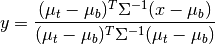
Adaptive Coherence/Cosine Estimator (ACE)
-
ace(X, target, background=None, window=None, cov=None, **kwargs)¶ Returns Adaptive Coherence/Cosine Estimator (ACE) detection scores.
Usage:
y = ace(X, target, background)
y = ace(X, target, window=<win> [, cov=<cov>])
Arguments:
X (numpy.ndarray):
For the first calling method shown, X can be an ndarray with shape (R, C, B) or an ndarray of shape (R * C, B). If the background keyword is given, it will be used for the image background statistics; otherwise, background statistics will be computed from X.
If the window keyword is given, X must be a 3-dimensional array and background statistics will be computed for each point in the image using a local window defined by the keyword.
target (ndarray or sequence of ndarray):
If X has shape (R, C, B), target can be any of the following:
A length-B ndarray. In this case, target specifies a single target spectrum to be detected. The return value will be an ndarray with shape (R, C).
An ndarray with shape (D, B). In this case, target contains D length-B targets that define a subspace for the detector. The return value will be an ndarray with shape (R, C).
A length-D sequence (e.g., list or tuple) of length-B ndarrays. In this case, the detector will be applied seperately to each of the D targets. This is equivalent to calling the function sequentially for each target and stacking the results but is much faster. The return value will be an ndarray with shape (R, C, D).
background (GaussianStats):
The Gaussian statistics for the background (e.g., the result of calling
calc_statsfor an image). This argument is not required if window is given.window (2-tuple of odd integers):
Must have the form (inner, outer), where the two values specify the widths (in pixels) of inner and outer windows centered about the pixel being evaulated. Both values must be odd integers. The background mean and covariance will be estimated from pixels in the outer window, excluding pixels within the inner window. For example, if (inner, outer) = (5, 21), then the number of pixels used to estimate background statistics will be
 . If this argument is given, background
is not required (and will be ignored, if given).
. If this argument is given, background
is not required (and will be ignored, if given).The window is modified near image borders, where full, centered windows cannot be created. The outer window will be shifted, as needed, to ensure that the outer window still has height and width outer (in this situation, the pixel being evaluated will not be at the center of the outer window). The inner window will be clipped, as needed, near image borders. For example, assume an image with 145 rows and columns. If the window used is (5, 21), then for the image pixel at (0, 0) (upper left corner), the the inner window will cover image[:3, :3] and the outer window will cover image[:21, :21]. For the pixel at (50, 1), the inner window will cover image[48:53, :4] and the outer window will cover image[40:51, :21].
cov (ndarray):
An optional covariance to use. If this parameter is given, cov will be used for all matched filter calculations (background covariance will not be recomputed in each window) and only the background mean will be recomputed in each window. If the window argument is specified, providing cov will allow the result to be computed much faster.
Keyword Arguments:
vectorize (bool, default True):
Specifies whether the function should attempt to vectorize operations. This typicall results in faster computation but will consume more memory.
Returns numpy.ndarray:
The return value will be the ACE scores for each input pixel. The shape of the returned array will be either (R, C) or (R, C, D), depending on the value of the target argument.
References:
Kraut S. & Scharf L.L., “The CFAR Adaptive Subspace Detector is a Scale- Invariant GLRT,” IEEE Trans. Signal Processing., vol. 47 no. 9, pp. 2538-41, Sep. 1999
AsterDatabase
-
class
AsterDatabase(sqlite_filename=None)¶ A relational database to manage ASTER spectral library data.
-
classmethod
create(filename, aster_data_dir=None)¶ Creates an ASTER relational database by parsing ASTER data files.
Arguments:
filename (str):
Name of the new sqlite database file to create.
aster_data_dir (str):
Path to the directory containing ASTER library data files. If this argument is not provided, no data will be imported.
Returns:
An
AsterDatabaseobject.Example:
>>> AsterDatabase.create("aster_lib.db", "/CDROM/ASTER2.0/data")
This is a class method (it does not require instantiating an AsterDatabase object) that creates a new database by parsing all of the files in the ASTER library data directory. Normally, this should only need to be called once. Subsequently, a corresponding database object can be created by instantiating a new AsterDatabase object with the path the database file as its argument. For example:
>>> from spectral.database.aster import AsterDatabase
>>> db = AsterDatabase("aster_lib.db")
-
create_envi_spectral_library(spectrumIDs, bandInfo)¶ Creates an ENVI-formatted spectral library for a list of spectra.
Arguments:
spectrumIDs (list of ints):
List of SpectrumID values for of spectra in the “Spectra” table of the ASTER database.
bandInfo (
BandInfo):The spectral bands to which the original ASTER library spectra will be resampled.
Returns:
A
SpectralLibraryobject.The IDs passed to the method should correspond to the SpectrumID field of the ASTER database “Spectra” table. All specified spectra will be resampled to the same discretization specified by the bandInfo parameter. See
spectral.BandResamplerfor details on the resampling method used.
-
get_signature(spectrumID)¶ Returns a spectrum with some additional metadata.
Usage:
sig = aster.get_signature(spectrumID)
Arguments:
spectrumID (int):
The SpectrumID value for the desired spectrum from the Spectra table in the database.
Returns:
sig (
Signature):An object with the following attributes:
Attribute
Type
Description
measurement_id
int
SpectrumID value from Spectra table
sample_name
str
Sample from the Samples table
sample_id
int
SampleID from the Samples table
x
list
list of band center wavelengths
y
list
list of spectrum values for each band
-
get_spectrum(spectrumID)¶ Returns a spectrum from the database.
Usage:
(x, y) = aster.get_spectrum(spectrumID)
Arguments:
spectrumID (int):
The SpectrumID value for the desired spectrum from the Spectra table in the database.
Returns:
x (list):
Band centers for the spectrum.
y (list):
Spectrum data values for each band.
Returns a pair of vectors containing the wavelengths and measured values values of a measurment. For additional metadata, call “get_signature” instead.
-
print_query(sql, args=None)¶ Prints the text result of an arbitrary SQL statement.
Arguments:
sql (str):
An SQL statement to be passed to the database. Use “?” for variables passed into the statement.
args (tuple):
Optional arguments which will replace the “?” placeholders in the sql argument.
This function performs the same query function as
spectral.database.Asterdatabase.queryexcept query results are printed to stdout instead of returning a cursor object.Example:
>>> sql = r'SELECT SpectrumID, Name FROM Samples, Spectra ' +
...        'WHERE Spectra.SampleID = Samples.SampleID ' +
...        'AND Name LIKE "%grass%" AND MinWavelength < ?'
>>> args = (0.5,)
>>> db.print_query(sql, args)
356|dry grass
357|grass
-
query(sql, args=None)¶ Returns the result of an arbitrary SQL statement.
Arguments:
sql (str):
An SQL statement to be passed to the database. Use “?” for variables passed into the statement.
args (tuple):
Optional arguments which will replace the “?” placeholders in the sql argument.
Returns:
An
sqlite3.Cursorobject with the query results.Example:
>>> sql = r'SELECT SpectrumID, Name FROM Samples, Spectra ' +
...        'WHERE Spectra.SampleID = Samples.SampleID ' +
...        'AND Name LIKE "%grass%" AND MinWavelength < ?'
>>> args = (0.5,)
>>> cur = db.query(sql, args)
>>> for row in cur:
...     print row
...
(356, u'dry grass')
(357, u'grass')
-
classmethod
BandInfo
-
class
BandInfo¶ A BandInfo object characterizes the spectral bands associated with an image. All BandInfo member variables are optional. For N bands, all members of type <list> will have length N and contain float values.
Member
Description
Default
centers
List of band centers
None
bandwidths
List of band FWHM values
None
centers_stdevs
List of std devs of band centers
None
bandwidth_stdevs
List of std devs of bands FWHMs
None
band_quantity
Image data type (e.g., “reflectance”)
“”
band_unit
Band unit (e.g., “nanometer”)
“”
BandResampler
-
class
BandResampler(centers1, centers2, fwhm1=None, fwhm2=None)¶ A callable object for resampling spectra between band discretizations.
A source band will contribute to any destination band where there is overlap between the FWHM of the two bands. If there is an overlap, an integral is performed over the region of overlap assuming the source band data value is constant over its FWHM (since we do not know the true spectral load over the source band) and the destination band has a Gaussian response function. Any target bands that do not have any overlapping source bands will contain NaN as the resampled band value.
If bandwidths are not specified for source or destination bands, the bands are assumed to have FWHM values that span half the distance to the adjacent bands.
-
__call__(spectrum)¶ Takes a source spectrum as input and returns a resampled spectrum.
Arguments:
spectrum (list or
numpy.ndarray):list or vector of values to be resampled. Must have same length as the source band discretiation used to created the resampler.
Returns:
A resampled rank-1
numpy.ndarraywith length corresponding to the destination band discretization used to create the resampler.Any target bands that do not have at lease one overlapping source band will contain float(‘nan’) as the resampled band value.
-
__init__(centers1, centers2, fwhm1=None, fwhm2=None)¶ BandResampler constructor.
Usage:
resampler = BandResampler(bandInfo1, bandInfo2)
resampler = BandResampler(centers1, centers2, [fwhm1 = None [, fwhm2 = None]])
Arguments:
bandInfo1 (
BandInfo):Discretization of the source bands.
bandInfo2 (
BandInfo):Discretization of the destination bands.
centers1 (list):
floats defining center values of source bands.
centers2 (list):
floats defining center values of destination bands.
fwhm1 (list):
Optional list defining FWHM values of source bands.
fwhm2 (list):
Optional list defining FWHM values of destination bands.
Returns:
A callable BandResampler object that takes a spectrum corresponding to the source bands and returns the spectrum resampled to the destination bands.
If bandwidths are not specified, the associated bands are assumed to have FWHM values that span half the distance to the adjacent bands.
-
Bhattacharyya Distance
-
bdist(class1, class2)¶ Calulates the Bhattacharyya distance between two classes.
USAGE: bd = bdist(class1, class2)
Arguments:
class1, class2 (
TrainingClass)Returns:
A float value for the Bhattacharyya Distance between the classes. This function is aliased to
bDistance.References:
Richards, J.A. & Jia, X. Remote Sensing Digital Image Analysis: An Introduction. (Springer: Berlin, 1999).
Note
Since it is unlikely anyone can actually remember how to spell “Bhattacharyya”, this function has been aliased to “bdist” for convenience.
calc_stats
-
calc_stats(image, mask=None, index=None, allow_nan=False)¶ Computes Gaussian stats for image data..
Arguments:
image (ndarrray,
Image, orspectral.Iterator):If an ndarray, it should have shape MxNxB and the mean & covariance will be calculated for each band (third dimension).
mask (ndarray):
If mask is specified, mean & covariance will be calculated for all pixels indicated in the mask array. If index is specified, all pixels in image for which mask == index will be used; otherwise, all nonzero elements of mask will be used.
index (int):
Specifies which value in mask to use to select pixels from image. If not specified but mask is, then all nonzero elements of mask will be used.
allow_nan (bool, default False):
If True, statistics will be computed even if np.nan values are present in the data; otherwise, ~spectral.algorithms.spymath.NaNValueError is raised.
If neither mask nor index are specified, all samples in vectors will be used.
Returns:
GaussianStats object:
This object will have members mean, cov, and nsamples.
covariance
-
covariance(*args)¶ Returns the covariance of the set of vectors.
Usage:
C = covariance(vectors [, mask=None [, index=None]])
Arguments:
vectors (ndarrray,
Image, orspectral.Iterator):If an ndarray, it should have shape MxNxB and the mean & covariance will be calculated for each band (third dimension).
mask (ndarray):
If mask is specified, mean & covariance will be calculated for all pixels indicated in the mask array. If index is specified, all pixels in image for which mask == index will be used; otherwise, all nonzero elements of mask will be used.
index (int):
Specifies which value in mask to use to select pixels from image. If not specified but mask is, then all nonzero elements of mask will be used.
If neither mask nor index are specified, all samples in vectors will be used.
Returns:
C (ndarray):
The BxB unbiased estimate (dividing by N-1) of the covariance of the vectors.
To also return the mean vector and number of samples, call
mean_covinstead.
cov_avg
-
cov_avg(image, mask, weighted=True)¶ Calculates the covariance averaged over a set of classes.
Arguments:
image (ndarrray,
Image, orspectral.Iterator):If an ndarray, it should have shape MxNxB and the mean & covariance will be calculated for each band (third dimension).
mask (integer-valued ndarray):
Elements specify the classes associated with pixels in image. All pixels associeted with non-zero elements of mask will be used in the covariance calculation.
weighted (bool, default True):
Specifies whether the individual class covariances should be weighted when computing the average. If True, each class will be weighted by the number of pixels provided for the class; otherwise, a simple average of the class covariances is performed.
Returns a class-averaged covariance matrix. The number of covariances used in the average is equal to the number of non-zero elements of mask.
EcostressDatabase
-
class
EcostressDatabase(sqlite_filename=None)¶ A relational database to manage ECOSTRESS spectral library data.
-
classmethod
create(filename, data_dir=None)¶ Creates an ECOSTRESS relational database by parsing ECOSTRESS data files.
Arguments:
filename (str):
Name of the new sqlite database file to create.
data_dir (str):
Path to the directory containing ECOSTRESS library data files. If this argument is not provided, no data will be imported.
Returns:
An
EcostressDatabaseobject.Example:
>>> EcostressDatabase.create("ecostress.db", "./eco_data_ver1/")
This is a class method (it does not require instantiating an EcostressDatabase object) that creates a new database by parsing all of the files in the ECOSTRESS library data directory. Normally, this should only need to be called once. Subsequently, a corresponding database object can be created by instantiating a new EcostressDatabase object with the path the database file as its argument. For example:
>>> from spectral.database.ecostress import EcostressDatabase
>>> db = EcostressDatabase("~/ecostress.db")
-
classmethod
FisherLinearDiscriminant
-
class
FisherLinearDiscriminant(vals, vecs, mean, cov_b, cov_w)¶ An object for storing a data set’s linear discriminant data. For C classes with B-dimensional data, the object has the following members:
eigenvalues:
A length C-1 array of eigenvalues
eigenvectors:
A BxC array of normalized eigenvectors
mean:
The length B mean vector of the image pixels (from all classes)
cov_b:
The BxB matrix of covariance between classes
cov_w:
The BxB matrix of average covariance within each class
transform:
A callable function to transform data to the space of the linear discriminant.
GaussianClassifier
-
class
GaussianClassifier(training_data=None, min_samples=None)¶ A Gaussian Maximum Likelihood Classifier
-
__init__(training_data=None, min_samples=None)¶ Creates the classifier and optionally trains it with training data.
Arguments:
training_data (
TrainingClassSet):The training classes on which to train the classifier.
min_samples (int) [default None]:
Minimum number of samples required from a training class to include it in the classifier.
-
classify_image(image)¶ Classifies an entire image, returning a classification map.
Arguments:
image (ndarray or
spectral.Image)The MxNxB image to classify.
Returns (ndarray):
An MxN ndarray of integers specifying the class for each pixel.
-
classify_spectrum(x)¶ Classifies a pixel into one of the trained classes.
Arguments:
x (list or rank-1 ndarray):
The unclassified spectrum.
Returns:
classIndex (int):
The index for the
TrainingClassto which x is classified.
-
train(training_data)¶ Trains the classifier on the given training data.
Arguments:
training_data (
TrainingClassSet):Data for the training classes.
-
GaussianStats
-
class
GaussianStats(mean=None, cov=None, nsamples=None, inv_cov=None)¶ A class for storing Gaussian statistics for a data set.
Statistics stored include:
mean:
Mean vector
cov:
Covariance matrix
nsamples:
Number of samples used in computing the statistics
Several derived statistics are computed on-demand (and cached) and are available as property attributes. These include:
inv_cov:
Inverse of the covariance
sqrt_cov:
Matrix square root of covariance: sqrt_cov.dot(sqrt_cov) == cov
sqrt_inv_cov:
Matrix square root of the inverse of covariance
log_det_cov:
The log of the determinant of the covariance matrix
principal_components:
The principal components of the data, based on mean and cov.
kmeans
-
kmeans(image, nclusters=10, max_iterations=20, **kwargs)¶ Performs iterative clustering using the k-means algorithm.
Arguments:
image (
numpy.ndarrayorspectral.Image):The MxNxB image on which to perform clustering.
nclusters (int) [default 10]:
Number of clusters to create. The number produced may be less than nclusters.
max_iterations (int) [default 20]:
Max number of iterations to perform.
Keyword Arguments:
start_clusters (
numpy.ndarray) [default None]:nclusters x B array of initial cluster centers. If not provided, initial cluster centers will be spaced evenly along the diagonal of the N-dimensional bounding box of the image data.
compare (callable object) [default None]:
Optional comparison function. compare must be a callable object that takes 2 MxN
numpy.ndarrayobjects as its arguments and returns non-zero when clustering is to be terminated. The two arguments are the cluster maps for the previous and current cluster cycle, respectively.distance (callable object) [default
L2]:The distance measure to use for comparison. The default is to use L2 (Euclidean) distance. For Manhattan distance, specify
L1.frames (list) [default None]:
If this argument is given and is a list object, each intermediate cluster map is appended to the list.
Returns a 2-tuple containing:
class_map (
numpy.ndarray):An MxN array whos values are the indices of the cluster for the corresponding element of image.
centers (
numpy.ndarray):An nclusters x B array of cluster centers.
Iterations are performed until clusters converge (no pixels reassigned between iterations), maxIterations is reached, or compare returns nonzero. If
KeyboardInterruptis generated (i.e., CTRL-C pressed) while the algorithm is executing, clusters are returned from the previously completed iteration.
linear_discriminant
-
linear_discriminant(classes, whiten=True)¶ Solve Fisher’s linear discriminant for eigenvalues and eigenvectors.
Usage: (L, V, Cb, Cw) = linear_discriminant(classes)
Arguments:
classes (
TrainingClassSet):The set of C classes to discriminate.
Returns a FisherLinearDiscriminant object containing the within/between- class covariances, mean vector, and a callable transform to convert data to the transform’s space.
This function determines the solution to the generalized eigenvalue problem
Cb * x = lambda * Cw * x
Since cov_w is normally invertable, the reduces to
(inv(Cw) * Cb) * x = lambda * x
References:
Richards, J.A. & Jia, X. Remote Sensing Digital Image Analysis: An Introduction. (Springer: Berlin, 1999).
LinearTransform
-
class
LinearTransform(A, **kwargs)¶ A callable linear transform object.
In addition to the __call__ method, which applies the transform to given, data, a LinearTransform object also has the following members:
dim_in (int):
The expected length of input vectors. This will be None if the input dimension is unknown (e.g., if the transform is a scalar).
dim_out (int):
The length of output vectors (after linear transformation). This will be None if the input dimension is unknown (e.g., if the transform is a scalar).
dtype (numpy dtype):
The numpy dtype for the output ndarray data.
-
__call__(X)¶ Applies the linear transformation to the given data.
Arguments:
X (
ndarrayor object with transform method):If X is an ndarray, it is either an (M,N,K) array containing M*N length-K vectors to be transformed or it is an (R,K) array of length-K vectors to be transformed. If X is an object with a method named transform the result of passing the LinearTransform object to the transform method will be returned.
Returns an (M,N,J) or (R,J) array, depending on shape of X, where J is the length of the first dimension of the array A passed to __init__.
-
__init__(A, **kwargs)¶ Arguments:
A (
ndarrray):An (J,K) array to be applied to length-K targets.
Keyword Argments:
pre (scalar or length-K sequence):
Additive offset to be applied prior to linear transformation.
post (scalar or length-J sequence):
An additive offset to be applied after linear transformation.
dtype (numpy dtype):
Explicit type for transformed data.
-
chain(transform)¶ Chains together two linear transforms. If the transform f1 is given by

and f2 by

then f1.chain(f2) returns a new LinearTransform, f3, whose output is given by
-
MahalanobisDistanceClassifier
-
class
MahalanobisDistanceClassifier(training_data=None, min_samples=None)¶ A Classifier using Mahalanobis distance for class discrimination
-
__init__(training_data=None, min_samples=None)¶ Creates the classifier and optionally trains it with training data.
Arguments:
training_data (
TrainingClassSet):The training classes on which to train the classifier.
min_samples (int) [default None]:
Minimum number of samples required from a training class to include it in the classifier.
-
classify_image(image)¶ Classifies an entire image, returning a classification map.
Arguments:
image (ndarray or
spectral.Image)The MxNxB image to classify.
Returns (ndarray):
An MxN ndarray of integers specifying the class for each pixel.
-
classify_spectrum(x)¶ Classifies a pixel into one of the trained classes.
Arguments:
x (list or rank-1 ndarray):
The unclassified spectrum.
Returns:
classIndex (int):
The index for the
TrainingClassto which x is classified.
-
train(trainingData)¶ Trains the classifier on the given training data.
Arguments:
trainingData (
TrainingClassSet):Data for the training classes.
-
map_class_ids
-
map_class_ids(src_class_image, dest_class_image, unlabeled=None)¶ Create a mapping between class labels in two classification images.
Running a classification algorithm (particularly an unsupervised one) multiple times on the same image can yield similar results but with different class labels (indices) for the same classes. This function produces a mapping of class indices from one classification image to another by finding class indices that share the most pixels between the two classification images.
Arguments:
src_class_image (ndarray):
An MxN integer array of class indices. The indices in this array will be mapped to indices in dest_class_image.
dest_class_image (ndarray):
An MxN integer array of class indices.
unlabeled (int or array of ints):
If this argument is provided, all pixels (in both images) will be ignored when counting coincident pixels to determine the mapping. If mapping a classification image to a ground truth image that has a labeled background value, set unlabeled to that value.
Return Value:
A dictionary whose keys are class indices from src_class_image and whose values are class indices from dest_class_image.
See also
map_classes
-
map_classes(class_image, class_id_map, allow_unmapped=False)¶ Modifies class indices according to a class index mapping.
Arguments:
class_image: (ndarray):
An MxN array of integer class indices.
class_id_map: (dict):
A dict whose keys are indices from class_image and whose values are new values for the corresponding indices. This value is usually the output of
map_class_ids.allow_unmapped (bool, default False):
A flag indicating whether class indices can appear in class_image without a corresponding key in class_id_map. If this value is False and an index in the image is found without a mapping key, a
ValueErroris raised. If True, the unmapped index will appear unmodified in the output image.Return Value:
An integer-valued ndarray with same shape as class_image
Example:
>>> m = spy.map_class_ids(result, gt, unlabeled=0)
>>> result_mapped = spy.map_classes(result, m)
See also
matched_filter
-
matched_filter(X, target, background=None, window=None, cov=None)¶ Computes a linear matched filter target detector score.
Usage:
y = matched_filter(X, target, background)
y = matched_filter(X, target, window=<win> [, cov=<cov>])
Given target/background means and a common covariance matrix, the matched filter response is given by:
where
 is the target mean,
  is the background
mean, and
is the background
mean, and  is the covariance.
Arguments:
X (numpy.ndarray):
For the first calling method shown, X can be an image with shape (R, C, B) or an ndarray of shape (R * C, B). If the background keyword is given, it will be used for the image background statistics; otherwise, background statistics will be computed from X.
If the window keyword is given, X must be a 3-dimensional array and background statistics will be computed for each point in the image using a local window defined by the keyword.
target (ndarray):
Length-K vector specifying the target to be detected.
background (GaussianStats):
The Gaussian statistics for the background (e.g., the result of calling
calc_statsfor an image). This argument is not required if window is given.window (2-tuple of odd integers):
Must have the form (inner, outer), where the two values specify the widths (in pixels) of inner and outer windows centered about the pixel being evaulated. Both values must be odd integers. The background mean and covariance will be estimated from pixels in the outer window, excluding pixels within the inner window. For example, if (inner, outer) = (5, 21), then the number of pixels used to estimate background statistics will be
. If this argument is given, background
is not required (and will be ignored, if given).The window is modified near image borders, where full, centered windows cannot be created. The outer window will be shifted, as needed, to ensure that the outer window still has height and width outer (in this situation, the pixel being evaluated will not be at the center of the outer window). The inner window will be clipped, as needed, near image borders. For example, assume an image with 145 rows and columns. If the window used is (5, 21), then for the image pixel at (0, 0) (upper left corner), the the inner window will cover image[:3, :3] and the outer window will cover image[:21, :21]. For the pixel at (50, 1), the inner window will cover image[48:53, :4] and the outer window will cover image[40:51, :21].
cov (ndarray):
An optional covariance to use. If this parameter is given, cov will be used for all matched filter calculations (background covariance will not be recomputed in each window) and only the background mean will be recomputed in each window. If the window argument is specified, providing cov will allow the result to be computed much faster.
Returns numpy.ndarray:
The return value will be the matched filter scores distance) for each pixel given. If X has shape (R, C, K), the returned ndarray will have shape (R, C).
MatchedFilter
-
class
MatchedFilter(background, target)¶ A callable linear matched filter.
Given target/background means and a common covariance matrix, the matched filter response is given by:
where
is the target mean, is the background
mean, and is the covariance.-
__call__(X)¶ Applies the linear transformation to the given data.
Arguments:
X (
ndarrayor object with transform method):If X is an ndarray, it is either an (M,N,K) array containing M*N length-K vectors to be transformed or it is an (R,K) array of length-K vectors to be transformed. If X is an object with a method named transform the result of passing the LinearTransform object to the transform method will be returned.
Returns an (M,N,J) or (R,J) array, depending on shape of X, where J is the length of the first dimension of the array A passed to __init__.
-
__init__(background, target)¶ Creates the filter, given background/target means and covariance.
Arguments:
background (GaussianStats):
The Gaussian statistics for the background (e.g., the result of calling
calc_stats).target (ndarray):
Length-K target mean
-
whiten(X)¶ Transforms data to the whitened space of the background.
Arguments:
X (ndarray):
Size (M,N,K) or (M*N,K) array of length K vectors to transform.
Returns an array of same size as X but linearly transformed to the whitened space of the filter.
-
mean_cov
-
mean_cov(image, mask=None, index=None)¶ Return the mean and covariance of the set of vectors.
Usage:
(mean, cov, S) = mean_cov(vectors [, mask=None [, index=None]])
Arguments:
image (ndarrray,
Image, orspectral.Iterator):If an ndarray, it should have shape MxNxB and the mean & covariance will be calculated for each band (third dimension).
mask (ndarray):
If mask is specified, mean & covariance will be calculated for all pixels indicated in the mask array. If index is specified, all pixels in image for which mask == index will be used; otherwise, all nonzero elements of mask will be used.
index (int):
Specifies which value in mask to use to select pixels from image. If not specified but mask is, then all nonzero elements of mask will be used.
If neither mask nor index are specified, all samples in vectors will be used.
Returns a 3-tuple containing:
mean (ndarray):
The length-B mean vectors
cov (ndarray):
The BxB unbiased estimate (dividing by N-1) of the covariance of the vectors.
S (int):
Number of samples used to calculate mean & cov
Calculate the mean and covariance of of the given vectors. The argument can be an Iterator, a SpyFile object, or an MxNxB array.
Minimum Noise Fraction (MNF)
-
mnf(signal, noise)¶ Computes Minimum Noise Fraction / Noise-Adjusted Principal Components.
Arguments:
signal (
GaussianStats):Estimated signal statistics
noise (
GaussianStats):Estimated noise statistics
Returns an
MNFResultobject, containing the Noise-Adjusted Principal Components (NAPC) and methods for denoising or reducing dimensionality of associated data.The Minimum Noise Fraction (MNF) is similar to the Principal Components transformation with the difference that the Principal Components associated with the MNF are ordered by descending signal-to-noise ratio (SNR) rather than overall image variance. Note that the eigenvalues of the NAPC are equal to one plus the SNR in the transformed space (since noise has whitened unit variance in the NAPC coordinate space).
Example:
>>> data = open_image('92AV3C.lan').load()
>>> signal = calc_stats(data)
>>> noise = noise_from_diffs(data[117: 137, 85: 122, :])
>>> mnfr = mnf(signal, noise)
>>> # De-noise the data by eliminating NAPC components where SNR < 10.
>>> # The de-noised data will be in the original coordinate space (at
>>> # full dimensionality).
>>> denoised = mnfr.denoise(data, snr=10)
>>> # Reduce dimensionality, retaining NAPC components where SNR >= 10.
>>> reduced = mnfr.reduce(data, snr=10)
>>> # Reduce dimensionality, retaining top 50 NAPC components.
>>> reduced = mnfr.reduce(data, num=50)
References:
Lee, James B., A. Stephen Woodyatt, and Mark Berman. “Enhancement of high spectral resolution remote-sensing data by a noise-adjusted principal components transform.” Geoscience and Remote Sensing, IEEE Transactions on 28.3 (1990): 295-304.
-
class
MNFResult(signal, noise, napc)¶ Result object returned by
mnf.This object contains data associates with a Minimum Noise Fraction calculation, including signal and noise statistics, as well as the Noise-Adjusted Principal Components (NAPC). This object can be used to denoise image data or to reduce its dimensionality.
-
denoise(X, **kwargs)¶ Returns a de-noised version of X.
Arguments:
X (np.ndarray):
Data to be de-noised. Can be a single pixel or an image.
One (and only one) of the following keywords must be specified:
num (int):
Number of Noise-Adjusted Principal Components to retain.
snr (float):
Threshold signal-to-noise ratio (SNR) to retain.
Returns denoised image data with same shape as X.
Note that calling this method is equivalent to calling the get_denoising_transform method with same keyword and applying the returned transform to X. If you only intend to denoise data with the same parameters multiple times, then it is more efficient to get the denoising transform and reuse it, rather than calling this method multilple times.
-
get_denoising_transform(**kwargs)¶ Returns a function for denoising image data.
One (and only one) of the following keywords must be specified:
num (int):
Number of Noise-Adjusted Principal Components to retain.
snr (float):
Threshold signal-to-noise ratio (SNR) to retain.
Returns a callable
LinearTransformobject for denoising image data.
-
get_reduction_transform(**kwargs)¶ Reduces dimensionality of image data.
One (and only one) of the following keywords must be specified:
num (int):
Number of Noise-Adjusted Principal Components to retain.
snr (float):
Threshold signal-to-noise ratio (SNR) to retain.
Returns a callable
LinearTransformobject for reducing the dimensionality of image data.
-
num_with_snr(snr)¶ Returns the number of components with SNR >= snr.
-
reduce(X, **kwargs)¶ Reduces dimensionality of image data.
Arguments:
X (np.ndarray):
Data to be reduced. Can be a single pixel or an image.
One (and only one) of the following keywords must be specified:
num (int):
Number of Noise-Adjusted Principal Components to retain.
snr (float):
Threshold signal-to-noise ratio (SNR) to retain.
Returns a verions of X with reduced dimensionality.
Note that calling this method is equivalent to calling the get_reduction_transform method with same keyword and applying the returned transform to X. If you intend to denoise data with the same parameters multiple times, then it is more efficient to get the reduction transform and reuse it, rather than calling this method multilple times.
-
msam
-
msam(data, members)¶ Modified SAM scores according to Oshigami, et al [1]. Endmembers are mean-subtracted prior to spectral angle calculation. Results are normalized such that the maximum value of 1 corresponds to a perfect match (zero spectral angle).
Arguments:
data (
numpy.ndarrayorspectral.Image):An MxNxB image for which spectral angles will be calculated.
members (
numpy.ndarray):CxB array of spectral endmembers.
Returns:
MxNxC array of MSAM scores with maximum value of 1 corresponding to a perfect match (zero spectral angle).
Calculates the spectral angles between each vector in data and each of the endmembers. The output of this function (angles) can be used to classify the data by minimum spectral angle by calling argmax(angles).
References:
[1] Shoko Oshigami, Yasushi Yamaguchi, Tatsumi Uezato, Atsushi Momose, Yessy Arvelyna, Yuu Kawakami, Taro Yajima, Shuichi Miyatake, and Anna Nguno. 2013. Mineralogical mapping of southern Namibia by application of continuum-removal MSAM method to the HyMap data. Int. J. Remote Sens. 34, 15 (August 2013), 5282-5295.
ndvi
-
ndvi(data, red, nir)¶ Calculates Normalized Difference Vegetation Index (NDVI).
Arguments:
data (ndarray or
spectral.Image):The array or SpyFile for which to calculate the index.
red (int or int range):
Index of the red band or an index range for multiple bands.
nir (int or int range):
An integer index of the near infrared band or an index range for multiple bands.
Returns an ndarray:
An array containing NDVI values in the range [-1.0, 1.0] for each corresponding element of data.
noise_from_diffs
-
noise_from_diffs(X, direction='lowerright')¶ Estimates noise statistcs by taking differences of adjacent pixels.
Arguments:
X (np.ndarray):
The data from which to estimage noise statistics. X should have shape (nrows, ncols, nbands).
direction (str, default “lowerright”):
The pixel direction along which to calculate pixel differences. Must be one of the following:
- ‘lowerright’:
Take difference with pixel diagonally to lower right
- ‘lowerleft’:
Take difference with pixel diagonally to lower right
- ‘right’:
Take difference with pixel to the right
- ‘lower’:
Take differenece with pixel below
Returns a
GaussianStatsobject.
orthogonalize
-
orthogonalize(vecs, start=0)¶ Performs Gram-Schmidt Orthogonalization on a set of vectors.
Arguments:
vecs (
numpy.ndarray):The set of vectors for which an orthonormal basis will be created. If there are C vectors of length B, vecs should be CxB.
start (int) [default 0]:
If start > 0, then vecs[start] will be assumed to already be orthonormal.
Returns:
A new CxB containing an orthonormal basis for the given vectors.
PerceptronClassifier
-
class
PerceptronClassifier(layers, k=1.0)¶ A multi-layer perceptron classifier with backpropagation learning.
Multi-layer perceptrons often require many (i.e., thousands) of iterations through the traning data to converge on a solution. Therefore, it is not recommended to attempt training a network on full-dimensional hyperspectral data or even on a full set of image pixels. It is likely preferable to first train the network on a subset of the data, then retrain the network (starting with network weights from initial training) on the full data set.
Example usage: Train an MLP with 20 samples from each training class after performing dimensionality reduction:
>>> classes = create_training_classes(data, gt)
>>> fld = linear_discriminant(classes)
>>> xdata = fld.transform(data)
>>> classes = create_training_classes(xdata, gt)
>>> nfeatures = xdata.shape[-1]
>>> nclasses = len(classes)
>>>
>>> p = PerceptronClassifier([nfeatures, 20, 8, nclasses])
>>> p.train(classes, 20, clip=0., accuracy=100., batch=1,
>>>         momentum=0.3, rate=0.3)
>>> c = p.classify(xdata)
-
classify(X, **kwargs)¶ Classifies the given sample. This has the same result as calling input and rounding the result.
-
classify_image(image)¶ Classifies an entire image, returning a classification map.
Arguments:
image (ndarray or
spectral.Image)The MxNxB image to classify.
Returns (ndarray):
An MxN ndarray of integers specifying the class for each pixel.
-
classify_spectrum(x)¶ Classifies a pixel into one of the trained classes.
Arguments:
x (list or rank-1 ndarray):
The unclassified spectrum.
Returns:
classIndex (int):
The index for the
TrainingClassto which x is classified.
-
input(x, clip=0.0)¶ Sets Perceptron input, activates neurons and sets & returns output.
Arguments:
x (sequence):
Inputs to input layer. Should not include a bias input.
clip (float >= 0):
Optional clipping value to limit sigmoid output. The sigmoid function has output in the range (0, 1). If the clip argument is set to a then all neuron outputs for the layer will be constrained to the range [a, 1 - a]. This can improve perceptron learning rate in some situations.
For classifying samples, call classify instead of input.
-
train(training_data, samples_per_class=0, *args, **kwargs)¶ Trains the Perceptron on the training data.
Arguments:
training_data (
TrainingClassSet):Data for the training classes.
samples_per_class (int):
Maximum number of training observations to user from each class in training_data. If this argument is not provided, all training data is used.
Keyword Arguments:
accuracy (float):
The percent training accuracy at which to terminate training, if the maximum number of iterations are not reached first. This value can be set greater than 100 to force a specified number of training iterations to be performed (e.g., to continue reducing the error term after 100% classification accuracy has been achieved.
rate (float):
The perceptron learning rate (typically in the range (0, 1]).
momentum (float):
The perceptron learning momentum term, which specifies the fraction of the previous update value that should be added to the current update term. The value should be in the range [0, 1).
batch (positive integer):
Specifies how many samples should be evaluated before an update is made to the perceptron weights. A value of 0 indicates batch updates should be performed (evaluate all training inputs prior to updating). Otherwise, updates will be aggregated for every batch inputs (i.e., batch == 1 is stochastic learning).
clip (float >= 0):
Optional clipping value to limit sigmoid output during training. The sigmoid function has output in the range (0, 1). If the clip argument is set to a then all neuron outputs for the layer will be constrained to the range [a, 1 - a]. This can improve perceptron learning rate in some situations.
After training the perceptron with a clipping value, train can be called again with clipping set to 0 to continue reducing the training error.
on_iteration (callable):
A callable object that accepts the perceptron as input and returns bool. If this argument is set, the object will be called at the end of each training iteration with the perceptron as its argument. If the callable returns True, training will terminate.
stdout:
An object with a write method that can be set to redirect training status messages somewhere other than stdout. To suppress output, set stdout to None.
Return value:
Returns True if desired accuracy was achieved.
Neural networks can require many iterations through a data set to converge. If convergence slows (as indicated by small changes in residual error), training can be terminated by pressing CTRL-C, which will preserve the network weights from the previous training iteration. train can then be called again with altered training parameters (e.g., increased learning rate or momentum) to increase the convergence rate.
-
Pixel Purity Index (PPI)
-
ppi(X, niters, threshold=0, centered=False, start=None, display=0, **imshow_kwargs)¶ Returns pixel purity indices for an image.
Arguments:
X (ndarray):
Image data for which to calculate pixel purity indices
niters (int):
Number of iterations to perform. Each iteration corresponds to a projection of the image data onto a random unit vector.
threshold (numeric):
If this value is zero, only the two most extreme pixels will have their indices incremented for each random vector. If the value is greater than zero, then all pixels whose projections onto the random vector are with threshold data units of either of the two extreme pixels will also have their indices incremented.
centered (bool):
If True, then the pixels in X are assumed to have their mean already subtracted; otherwise, the mean of X will be computed and subtracted prior to computing the purity indices.
start (ndarray):
An optional array of initial purity indices. This can be used to continue computing PPI values after a previous call to ppi (i.e., set start equal to the return value from a previou call to ppi. This should be an integer-valued array whose dimensions are equal to the first two dimensions of X.
display (integer):
If set to a postive integer, a
ImageViewwindow will be opened and dynamically display PPI values as the function iterates. The value specifies the number of PPI iterations between display updates. It is recommended to use a value around 100 or higher. If the stretch keyword (seeget_rgbfor meaning) is not provided, a default stretch of (0.99, 0.999) is used.Return value:
An ndarray of integers that represent the pixel purity indices of the input image. The return array will have dimensions equal to the first two dimensions of the input image.
Keyword Arguments:
Any keyword accepted by
imshow. These keywords will be passed to the image display and only have an effect if the display argument is nonzero.This function can be interruped with a KeyboardInterrupt (ctrl-C), in which case, the most recent value of the PPI array will be returned. This can be used in conjunction with the display argument to view the progression of the PPI values until they appear stable, then terminate iteration using ctrl-C.
References:
Boardman J.W., Kruse F.A, and Green R.O., “Mapping Target Signatures via Partial Unmixing of AVIRIS Data,” Pasadena, California, USA, 23 Jan 1995, URI: http://hdl.handle.net/2014/33635
principal_components
-
principal_components(image)¶ Calculate Principal Component eigenvalues & eigenvectors for an image.
Usage:
pc = principal_components(image)
Arguments:
image (ndarray,
spectral.Image,GaussianStats):An MxNxB image
Returns a
PrincipalComponentsobject with the following members:eigenvalues:
A length B array of eigenvalues
eigenvectors:
A BxB array of normalized eigenvectors
stats (
GaussianStats):A statistics object containing mean, cov, and nsamples.
transform:
A callable function to transform data to the space of the principal components.
reduce:
A method to reduce the number of eigenvalues.
denoise:
A callable function to denoise data using a reduced set of principal components.
get_denoising_transform:
A callable function that returns a function for denoising data.
PrincipalComponents
-
class
PrincipalComponents(vals, vecs, stats)¶ An object for storing a data set’s principal components. The object has the following members:
eigenvalues:
A length B array of eigenvalues sorted in descending order
eigenvectors:
A BxB array of normalized eigenvectors (in columns)
stats (
GaussianStats):A statistics object containing mean, cov, and nsamples.
transform:
A callable function to transform data to the space of the principal components.
reduce:
A method to return a reduced set of principal components based on either a fixed number of components or a fraction of total variance.
denoise:
A callable function to denoise data using a reduced set of principal components.
get_denoising_transform:
A callable function that returns a function for denoising data.
-
denoise(X, **kwargs)¶ Returns a de-noised version of X.
Arguments:
X (np.ndarray):
Data to be de-noised. Can be a single pixel or an image.
Keyword Arguments (one of the following must be specified):
num (integer):
Number of eigenvalues/eigenvectors to use. The top num eigenvalues will be used.
eigs (list):
A list of indices of eigenvalues/eigenvectors to be used.
fraction (float):
The fraction of total image variance to retain. Eigenvalues will be included (starting from greatest to smallest) until fraction of total image variance is retained.
Returns denoised image data with same shape as X.
Note that calling this method is equivalent to calling the get_denoising_transform method with same keyword and applying the returned transform to X. If you only intend to denoise data with the same parameters multiple times, then it is more efficient to get the denoising transform and reuse it, rather than calling this method multilple times.
-
get_denoising_transform(**kwargs)¶ Returns a function for denoising image data.
Keyword Arguments (one of the following must be specified):
num (integer):
Number of eigenvalues/eigenvectors to use. The top num eigenvalues will be used.
eigs (list):
A list of indices of eigenvalues/eigenvectors to be used.
fraction (float):
The fraction of total image variance to retain. Eigenvalues will be included (starting from greatest to smallest) until fraction of total image variance is retained.
Returns a callable
LinearTransformobject for denoising image data.
-
reduce(N=0, **kwargs)¶ Reduces the number of principal components.
Keyword Arguments (one of the following must be specified):
num (integer):
Number of eigenvalues/eigenvectors to retain. The top num eigenvalues will be retained.
eigs (list):
A list of indices of eigenvalues/eigenvectors to be retained.
fraction (float):
The fraction of total image variance to retain. Eigenvalues will be retained (starting from greatest to smallest) until fraction of total image variance is retained.
-
RX Anomaly Detector
-
rx(X, background=None, window=None, cov=None)¶ Computes RX anomaly detector scores.
Usage:
y = rx(X [, background=bg])
y = rx(X, window=(inner, outer) [, cov=C])
The RX anomaly detector produces a detection statistic equal to the squared Mahalanobis distance of a spectrum from a background distribution according to
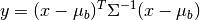
where x is the pixel spectrum,
is the background
mean, and is the background covariance.Arguments:
X (numpy.ndarray):
For the first calling method shown, X can be an image with shape (R, C, B) or an ndarray of shape (R * C, B). If the background keyword is given, it will be used for the image background statistics; otherwise, background statistics will be computed from X.
If the window keyword is given, X must be a 3-dimensional array and background statistics will be computed for each point in the image using a local window defined by the keyword.
background (GaussianStats):
The Gaussian statistics for the background (e.g., the result of calling
calc_stats). If no background stats are provided, they will be estimated based on data passed to the detector.window (2-tuple of odd integers):
Must have the form (inner, outer), where the two values specify the widths (in pixels) of inner and outer windows centered about the pixel being evaulated. Both values must be odd integers. The background mean and covariance will be estimated from pixels in the outer window, excluding pixels within the inner window. For example, if (inner, outer) = (5, 21), then the number of pixels used to estimate background statistics will be
.The window are modified near image borders, where full, centered windows cannot be created. The outer window will be shifted, as needed, to ensure that the outer window still has height and width outer (in this situation, the pixel being evaluated will not be at the center of the outer window). The inner window will be clipped, as needed, near image borders. For example, assume an image with 145 rows and columns. If the window used is (5, 21), then for the image pixel at (0, 0) (upper left corner), the the inner window will cover image[:3, :3] and the outer window will cover image[:21, :21]. For the pixel at (50, 1), the inner window will cover image[48:53, :4] and the outer window will cover image[40:51, :21].
cov (ndarray):
An optional covariance to use. If this parameter is given, cov will be used for all RX calculations (background covariance will not be recomputed in each window) and only the background mean will be recomputed in each window.
Returns numpy.ndarray:
The return value will be the RX detector score (squared Mahalanobis distance) for each pixel given. If X has shape (R, C, B), the returned ndarray will have shape (R, C)..
References:
Reed, I.S. and Yu, X., “Adaptive multiple-band CFAR detection of an optical pattern with unknown spectral distribution,” IEEE Trans. Acoust., Speech, Signal Processing, vol. 38, pp. 1760-1770, Oct. 1990.
spectral_angles
-
spectral_angles(data, members)¶ Calculates spectral angles with respect to given set of spectra.
Arguments:
data (
numpy.ndarrayorspectral.Image):An MxNxB image for which spectral angles will be calculated.
members (
numpy.ndarray):CxB array of spectral endmembers.
Returns:
MxNxC array of spectral angles.
Calculates the spectral angles between each vector in data and each of the endmembers. The output of this function (angles) can be used to classify the data by minimum spectral angle by calling argmin(angles).
SpectralLibrary
-
class
SpectralLibrary(data, header=None, params=None) The envi.SpectralLibrary class holds data contained in an ENVI-formatted spectral library file (.sli files), which stores data as specified by a corresponding .hdr header file. The primary members of an Envi.SpectralLibrary object are:
spectra (
numpy.ndarray):A subscriptable array of all spectra in the library. spectra will have shape CxB, where C is the number of spectra in the library and B is the number of bands for each spectrum.
names (list of str):
A length-C list of names corresponding to the spectra.
bands (
spectral.BandInfo):Spectral bands associated with the library spectra.
-
save(file_basename, description=None) Saves the spectral library to a library file.
Arguments:
file_basename (str):
Name of the file (without extension) to save.
description (str):
Optional text description of the library.
This method creates two files: file_basename.hdr and file_basename.sli.
-
transform_image
-
transform_image(transform, img)¶ Applies a linear transform to an image.
Arguments:
transform (ndarray or LinearTransform):
The CxB linear transform to apply.
img (ndarray or
spectral.SpyFile):The MxNxB image to be transformed.
Returns (ndarray or :class:spectral.spyfile.TransformedImage`):
The transformed image.
If img is an ndarray, then a MxNxC ndarray is returned. If img is a
spectral.SpyFile, then aspectral.spyfile.TransformedImageis returned.
Configuration
SpySettings
-
class
SpySettings¶ Run-time settings for the spectral module.
After importing spectral, the settings object is referenced as spectral.settings.
Noteworthy members:
WX_GL_DEPTH_SIZE (integer, default 24):
Sets the depth (in number of bits) for the OpenGL depth buffer. If calls to view_cube or view_nd result in windows with blank canvases, try reducing this value.
envi_support_nonlowercase_params (bool, default False)
By default, ENVI headers are read with parameter names converted to lower case. If this attribute is set to True, parameters will be read with original capitalization retained.
show_progress (bool, default True):
Indicates whether long-running algorithms should display progress to sys.stdout. It can be useful to set this value to False when SPy is embedded in another application (e.g., IPython Notebook).
imshow_figure_size (2-tuple of integers, default None):
Width and height (in inches) of windows opened with imshow. If this value is None, matplotlib’s default size is used.
imshow_background_color (3-tuple of integers, default (0,0,0)):
Default color to use for masked pixels in imshow displays.
imshow_interpolation (str, default None):
Pixel interpolation to be used in imshow windows. If this value is None, matplotlib’s default interpolation is used. Note that zoom windows always use “nearest” interpolation.
imshow_stretch:
Default RGB linear color stretch to perform.
imshow_stretch_all:
If True, each color channel limits are determined independently.
imshow_zoom_figure_width (int, default None):
Width of zoom windows opened from an imshow window. Since zoom windows are always square, this is also the window height. If this value is None, matplotlib’s default window size is used.
imshow_zoom_pixel_width (int, default 50):
Number of source image pixel rows and columns to display in a zoom window.
imshow_float_cmap (str, default “gray”):
imshow color map to use with floating point arrays.
imshow_class_alpha (float, default 0.5):
alpha blending value to use for imshow class overlays
imshow_enable_rectangle_selector (bool, default True):
Whether to create the rectangle selection tool that enables interactive image pixel class labeling. On some OS/backend combinations, an exception may be raised when this object is created so disabling it allows imshow windows to be created without using the selector tool.
imshow_disable_mpl_callbacks (bool, default True):
If True, several matplotlib keypress event callbacks will be disabled to prevent conflicts with callbacks from SPy. The matplotlib callbacks can be set back to their defaults by calling matplotlib.rcdefaults().
Utilities
iterator
-
iterator(image, mask=None, index=None)¶ Returns an iterator over pixels in the image.
Arguments:
image (ndarray or
spectral.Image):An image over whose pixels will be iterated.
mask (ndarray) [default None]:
An array of integers that specify over which pixels in image iteration should be performed.
index (int) [default None]:
Specifies which value in mask should be used for iteration.
Returns (
spectral.Iterator):An iterator over image pixels.
If neither mask nor index are defined, iteration is performed over all pixels. If mask (but not index) is defined, iteration is performed over all pixels for which mask is nonzero. If both mask and index are defined, iteration is performed over all pixels image[i,j] for which mask[i,j] == index.