Displaying Data

Starting IPython

SPy uses IPython to provide GUI windows without blocking the interactive python interpreter. To enable this, you must start IPython in “pylab” mode. If you have already set your matplotlib backend to either “WX” or “WXAgg” (see note below) in your matplotlibrc file, you should be able to start IPython for SPy like this:

ipython --pylab

You can also set the backend explicitly when starting IPython this way:

ipython --pylab=wx

Note

If you are not calling GUI functions (calling save_rgb doesn’t count as a GUI function), then it is not necessary to run IPython - you can run the standard python interpreter.

Note

If you are not able to run the WX backend on your system, you can still use a different backend (e.g., Qt4Agg or TkAgg); however you will be unable to call the view_cube or view_nd functions.

Raster Displays

The SPy imshow function is a wrapper around the matplotlib function of the same name. The main differences are that the SPy version makes it easy to display bands from multispectral/hyperspectral images, it renders classification images, and supports several additional types of interactivity.

Image Data Display

The imshow function produces a raster display of data associated with an np.ndarray or SpyFile object.

In [1]: from spectral import *

In [2]: img = open_image('92AV3C.lan')

In [3]: view = imshow(img, (29, 19, 9))

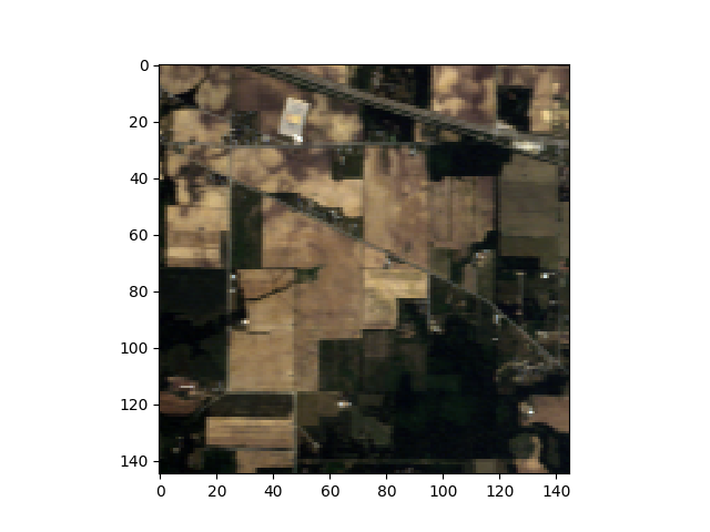
When displaying the image interactively, the matplotlib button controls can be used to pan and zoom the displayed images. If you press the “z” keyboard key, a zoom window will be opened, which displays a magnified view of the image. By holding down the CONTROL key and left-clicking in the original window, the zoom window will pan to the pixel clicked in the original window.

Changed in version 0.16.0: By default, imshow function applies a linear histogram stretch of the RGB display data. The the color stretch can be controlled by the stretch, bounds, and stretch_all keyword to the imshow function (see get_rgb for the meaning of these keywords). To adjust the color stretch of a displayed image, the set_rgb_options method of the ImageView object can be called.

RGB data limits for a displayed image can be printed from the __str__ method of the ImageView object:

In [4]: print(view)
ImageView object:
  Display bands       :  (29, 19, 9)
  Interpolation       :  <default>
  RGB data limits     :
    R: [2054.0, 6317.0]
    G: [2775.0, 7307.0]
    B: [3560.0, 7928.0]

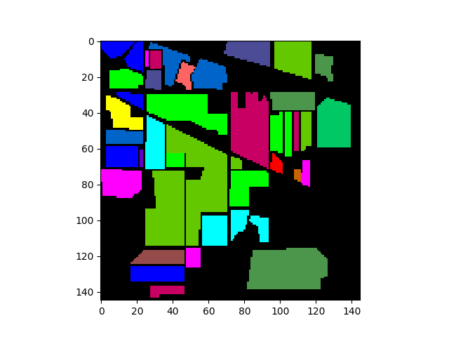
Class Map Display

To display the ground truth image using imshow, set the classes argument in the imshow function:

In [5]: gt = open_image('92AV3GT.GIS').read_band(0)

In [6]: view = imshow(classes=gt)

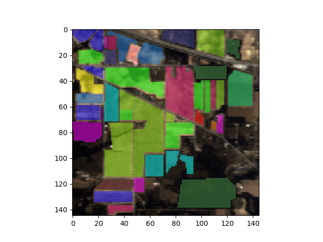
It is also possible to switch between displaying image bands and class colors, as well as displaying class color masks overlayed on the image data display. To do this, specify both the data and class values when calling imshow:

In [7]: view = imshow(img, (30, 20, 10), classes=gt)

The default display mode is to show the image bands. Press “d”, “c”, or “C” (while focus is on the image window) to switch the display to data, classes, or class overlay, respectively. Setting the display parameters can also be done programatically. For example, to display the image with overlayed class masks, using an alpha transparency of 0.5, type the following commands after calling imshow:

In [8]: view = imshow(img, (30, 20, 10), classes=gt)

In [9]: view.set_display_mode('overlay')

In [10]: view.class_alpha = 0.5

Interactive Class Labeling

The ImageView window provides the ability to modify pixel class IDs interactively by selecting rectangular regions in the image and assigning a new class ID. Applying a class ID to a rectangular region is done using the following steps:

1. Call imshow, providing an initial array for the classes argument. This must be a non-negative, integer-valued array. A class ID value of zero represents an unlabeled pixel so to start with a completely unlabeled image, pass an array of all zeros for the classes argument.

2. While holding the SHIFT key, click with the left mouse button at the upper left corner of the rectangle to be selected. Drag the mouse cursor and release the mouse button at the lower right corner of the rectangular region. Note that releasing the SHIFT key before the mouse button is released will result in cancellation of the selection operation.

3. With focus still on the ImageView window, enter the numeric class ID to apply to the region. The class ID can contain multiple digits. The digits will not be echoed on the command line. Press ENTER to apply the class ID. The command line will request confirmation of the opertion. Press ENTER again to apply the class ID or press any other key to cancel the operation.

Classes can be assigned form either a main ImageView window or from an associated zoom window. While the selection tool only produces rectangular regions, you can assign classes to non-rectangular regions by first assigning the class ID to a super-rectangle covering all the pixels of interest, then reassigning sub-rectangles back to class 0 (or whatever was the original class ID).

Additional Capabilities

To get help on ImageView keyboard & mouse functions, press “h” while focus is on the image window to display all keybinds and mouse functions:

Mouse Functions:
----------------
ctrl+left-click          ->   pan zoom window to pixel
shift+left-click&drag    ->   select rectangular image region
left-dblclick            ->   plot pixel spectrum

Keybinds:
---------
0-9     -> enter class ID for image pixel labeling
ENTER   -> apply specified class ID to selected rectangular region
a/A     -> decrease/increase class overlay alpha value
c       -> set display mode to "classes" (if classes set)
C       -> set display mode to "overlay" (if data and classes set)
d       -> set display mode to "data" (if data set)
h       -> print help message
i       -> toggle pixel interpolation between "nearest" and SPy default.
z       -> open zoom window

See matplotlib imshow documentation for addition key binds.

To customize behavior of the image display beyond what is provided by the imshow function, you can create an ImageView object directly and customize it prior to calling its show method. You can also access the matplotlib figure and canvas attributes from the axes attribute of the ImageView object returned by imshow. Finally, you can customize some of the default behaviours of the image display by modifiying members of the module’s SpySettings object.

Saving RGB Image Files

To save an image display to a file, use the save_rgb function, which uses the same arguments as imshow but with the saved image file name as the first argument.

In [11]: save_rgb('rgb.jpg', img, [29, 19, 9])

Saving an indexed color image is similar to saving an RGB image; however, save_rgb is unable to determine if the image being saved is a single-band (greyscale) image or an indexed color image. Therefore, to save as an indexed color image, the color palette must be explicitly passed as a keyword argument:

In [12]: save_rgb('gt.jpg', gt, colors=spy_colors)

Spectrum Plots

The image display windows provide a few interactive functions. If you create an image display with imshow (or view) and then double-click on a particular location in the window, a new window will be created with a 2D plot of the spectrum for the pixel that was clicked. It should look something like this:

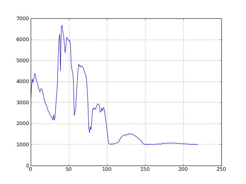
Note that the row/col of the double-clicked pixel is printed on the command prompt. Since there is no spectral band metadata in our sample image file, the spectral plot’s axes are unlabeled and the pixel band values are plotted vs. band number, rather than wavelength. To have the data plotted vs. wavelength, we must first associated spectral band information with the image.

In [13]: import spectral.io.aviris as aviris

In [14]: img.bands = aviris.read_aviris_bands('92AV3C.spc')

Now, close the image and spectral plot windows, call view again and click on a few locations in the image display. You will notice that the x-axis now shows the wavelengths associated with each band.

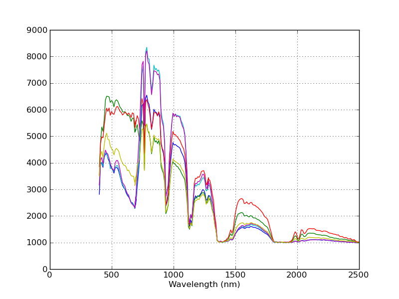
Notice that the spectra are now plotted against their associated wavelengths.

The spectral plots are intended as a convenience to enable one to quickly view spectra from an image. If you would like a prettier plot of the same data, you can use SPy to read the spectra from the image and create a customized plot by using matplotlib directly.

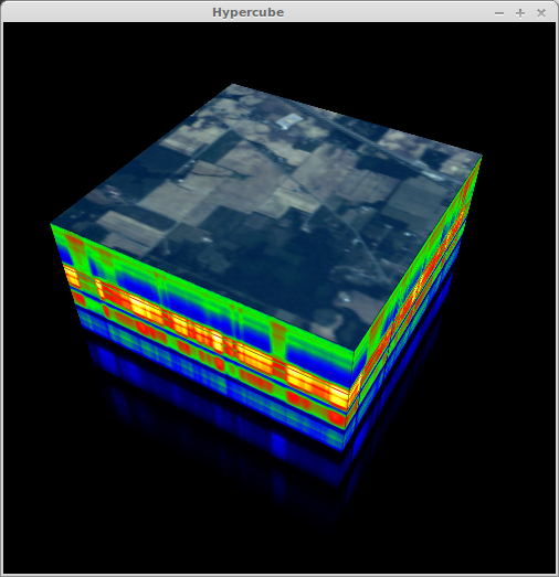
Hypercube Display

In the context of hyperspectral imagery, a 3D hypercube is a 3-dimensional representation of a hyperspectral image where the x and y dimensions are the spatial dimensions of the image and the third dimension is the spectral dimension. The analytical utility of hypercube displays is debatable but what is not debatable is that they look extremely cool.

After calling view_cube, a new window will open with the 3D hypercube displayed. After shifting command focus to the newly created window, you can use keyboard input to alter the view of the hypercube. Using keyword arguments, you can change the image displayed on the top of the cube, as well as the color scale used on the sides of of the cube.

In [15]: view_cube(img, bands=[29, 19, 9])

Mouse Functions:
----------------
left-click & drag        ->   Rotate cube
CTRL+left-click & drag   ->   Zoom in/out
SHIFT+left-click & drag  ->  Pan

Keybinds:
---------
l       -> toggle light
t/g     -> stretch/compress z-dimension
h       -> print help message
q       -> close window

Note

If the window opened by view_cube produces a blank canvas (no cube is displayed), it may be due to your display adapter not supporting a 32-bit depth buffer. You can reduce the size of the depth buffer used by view_cube and view_nd to a smaller value (e.g., 16) by issuing the following commands:

In [16]: import spectral

In [17]: spectral.settings.WX_GL_DEPTH_SIZE = 16

N-Dimensional Feature Display

Since hyperspectral images contain hundreds of narrow, contiguous bands, there is often strong correlation between bands (particularly adjacent bands). To increase the amount of information displayed, it is common to reduce the dimensionality of the image to a smaller set of features with higher information density (e.g., by principal components transformation). Nevertheless, there are typically still many more than three features remaining in the transformed image so the analyst must decide which are the “best” three features to display to highlight some aspect of the data set (e.g., separability of the spectral classes). It is desirable to be able to quickly switch displayed features to examine many combinations of features in a short time span.

In most cases, the display will be more useful by first performing dimensionality reduction prior to viewint the data (e.g., by selecting some number of principal components).

In [18]: data = open_image('92AV3C.lan').load()

In [19]: gt = open_image('92AV3GT.GIS').read_band(0)

In [20]: pc = principal_components(data)
Covariance.....done

In [21]: xdata = pc.transform(data)

In [22]: w = view_nd(xdata[:,:,:15], classes=gt)

A new window should open and appear as follows:

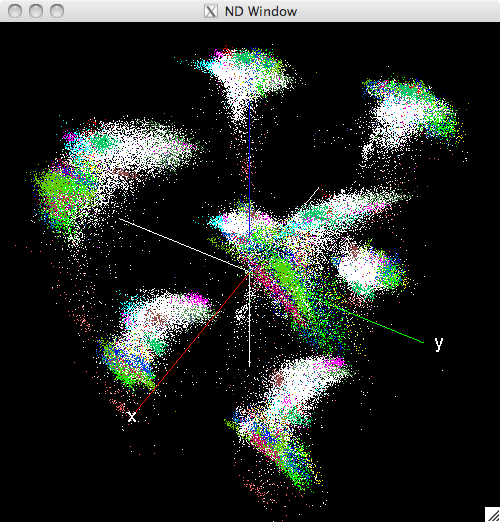
Initial view of the N-Dimensinal window

The python prompt will display the set of keyboard and mouse commands accepted by the ND window:

Mouse functions:
---------------
Left-click & drag       -->     Rotate viewing geometry (or pan)
CTRL+Left-click & drag  -->     Zoom viewing geometry
CTRL+SHIFT+Left-click   -->     Print image row/col and class of selected pixel
SHIFT+Left-click & drag -->     Define selection box in the window
Right-click             -->     Open GLUT menu for pixel reassignment

Keyboard functions:
-------------------
a       -->     Toggle axis display
c       -->     View dynamic raster image of class values
d       -->     Cycle display mode between single-quadrant, mirrored octants,
                and independent octants (display will not change until features
                are randomzed again)
f       -->     Randomize features displayed
h       -->     Print this help message
m       -->     Toggle mouse function between rotate/zoom and pan modes
p/P     -->     Increase/Decrease the size of displayed points
q       -->     Exit the application
r       -->     Reset viewing geometry
u       -->     Toggle display of unassigned points (points with class == 0)

The following figure shows the same window after the display has been rotated, unlabeled pixels (white) have been supressed, and the displayed pixel size has been increased:

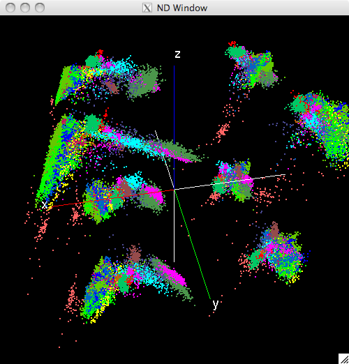
Modified view of the N-Dimensinal window

Display Modes

To facilitate interactive visual analysis of high-dimensional images, the view_nd function provides several modes for displaying high-dimensional data in a 3-dimensional display window:

1. Single-Octant Mode - In this mode, three features from the image are selected and mapped to the x, y, and z axes in the 3D window. The data are translated and scaled such that the displayed points fill the positive x/y/z octant of the 3D space. The user can choose to randomly select a new set of three features to display. With this randomization capability, the user can rapidly cycle through various combinations of features to identify desirable projections.

2. Mirrored-Octant Mode - In this mode, three features are mapped to the positive x, y, and z axes as in the single-octant mode. However, an additional three features are selected and mapped the the negative portions of the x, y, and z axes. The image pixels are then displayed in each of the eight octants of the 3D display, using whichever features are associated with the three semi-axes for the particular octant. In this mode, each partial plane defined by two semi-axes can be considered a mirror, with the two perpendicular semi-axes representing different features. For example, if the x, y, z, -x, -y, and -z semi-axes are associated with features 1 through 6, respectively, then the data points in the x/y/z and x/y/-z quadrants will have a common projection onto the x/y plane. However, since z and -z are mapped to different features, the data points will have different projections along the z and -z axes. As with the single-octant mode, the user can randomize the 6 features displayed.

3. Independent-Octant Mode - In this mode, each octant of the 3D space represents 3 independent features, enabling up to 24 features to be displayed. As with the other two modes, the data points are translated and scaled such that the entire set of image pixels completely fills each octant. It is possible that a particular feature may be used in more than one octant.

The user has the option of switching between display modes. Which display mode is best may depend on a number of factors relating to the data set used or the system on which the application is run. For images with sufficiently large numbers of pixels, the system’s display refresh rate may begin to suffer in mirrored-octant or independent-octant mode because each image pixel must be rendered 8 times. When performance is not an issue, the latter two modes provide more simultaneous projections of the data that may enable a user to more quickly explore the data set.

User Interaction

The initial 3D view of the rendered image data will almost certainly not be the ideal 3D viewing geometry; therefore, the window allows the user to manipulate the view by using the mouse input to zoom, pan, and rotate the viewing geometry. The user can also increase/decrease the size of displayed image pixels and toggle display of unlabeled (class 0) pixels.

While pixel color allows the user to distinguish between classes of displayed pixels, it may not be obvious to which class a given color is associated. To identify the class of a specific pixel, the user can click on a pixel and the python command line will print the pixel’s location within the image (row and column values) and the number (ID) of the class of the pixel. Since clicking on a single screen pixel is difficult, the user can first increase the size of the displayed image pixels such that the image pixel can easily be selected with the mouse.

Data Manipulation

It is common for an analyst to want to review the results of unsupervised classification and subsequently combine pixel classes or reassign pixels to new or different classes. Similarly, an analyst may want to assess ground truth data and possibly reassign pixels that were erroneously included in a class when the ground truth image was developed. To support this capability, the N-D window allows the user to click and drag with the mouse to select a rectangular region and then reassign all pixels lying within the defined box. The application will not only reassign the pixels visible within the selection box but also all pixels within the projection of the box through the 3D space.

When view_nd is called, it returns a proxy object that has a classes member that represents the current array of class values associated with the ND display. The proxy object can be used to access the updated class array after image pixels have been reassigned through the ND window. The proxy object also has a set_features method to specify the set of features displayed in the 3D window.

Tip

Before reassigning pixel class values, press the “c” key to open a second window displaying a raster view of the current image pixel class values. Then, when you reassign pixel classes in the ND window, the class raster view will update automatically, providing and indication of which pixels in the source image were modified.