Spectral Libraries
ECOSTRESS Spectral Library
The ECOSTRESS spectral library provides over 3,000 high-resolution spectra for numerous classes of materials [Meerdink2019]. The spectra and associated metadata are provided as a large set of ASCII text files. SPy provides the ability to import the ECOSTRESS library spectra and a subset of the associated metadata into a relational databased that can be easily accessed from Python.
You will first need to get a copy of the ECOSTRESS spectral library data files,
which can be requested here. Once you have
acquired the library data, you can import the data in to an sqlite
database as follows:
In [1]: db = spy.EcostressDatabase.create('ecostress.db', './eco_data_ver1')
Importing ./eco_data_ver1/vegetation.tree.betula.lenta.tir.bele-1-55.ucsb.nicolet.spectrum.txt.
Importing ./eco_data_ver1/vegetation.tree.quercus.lobata.tir.vh282.ucsb.nicolet.spectrum.txt.
Importing ./eco_data_ver1/nonphotosyntheticvegetation.branches.adenostoma.fasciculatum.vswir.vh334.ucsb.asd.spectrum.txt.
Importing ./eco_data_ver1/mineral.silicate.cyclosilicate.fine.tir.cs-2a.jpl.nicolet.spectrum.txt.
Importing ./eco_data_ver1/mineral.hydroxide.none.fine.tir.goethite_1.jhu.nicolet.spectrum.txt.
---// snip //---
Importing ./eco_data_ver1/mineral.silicate.inosilicate.coarse.vswir.in-8a.jpl.perkin.spectrum.txt.
Importing ./eco_data_ver1/vegetation.shrub.aloe.arborescens.tir.jpl077.jpl.nicolet.spectrum.txt.
Importing ./eco_data_ver1/mineral.silicate.phyllosilicate.coarse.tir.ps-12f.jpl.nicolet.spectrum.txt.
Processed 3403 files.
Note
The ECOSTRESS library supercedes the older ASTER spectral library
[Baldridge2009]. To import data from version 2.0 of the ASTER library,
follow the precedure above but with AsterDatabase instead of
EcostressDatabase.
Once the database has been created, it can be accessed by instantiating an
EcostressDatabase object for the database file (it can also be
accessed by using sqlite external to Python). The current implementation of the
SPy database contains two tables: Samples and Spectra. There is a one-to-one
relationship between rows in the two tables but they have been separate to support
potential future changes to the database. The schemas for the tables are in the
schemas attribute of the database object:
In [2]: db = EcostressDatabase('ecostress.db')

In [3]: for s in db.schemas:
   ...:     print(s)
   ...:
CREATE TABLE Samples (SampleID INTEGER PRIMARY KEY, Name TEXT, Type TEXT, Class TEXT, SubClass TEXT, ParticleSize TEXT, SampleNum TEXT, Owner TEXT, Origin TEXT, Phase TEXT, Description TEXT)
CREATE TABLE Spectra (SpectrumID INTEGER PRIMARY KEY, SampleID INTEGER, SensorCalibrationID INTEGER, Instrument TEXT, Environment TEXT, Measurement TEXT, XUnit TEXT, YUnit TEXT, MinWavelength FLOAT, MaxWavelength FLOAT, NumValues INTEGER, XData BLOB, YData BLOB)
Descriptions of most of the Sample table columns can be found in the ECOSTRESS
Spectral Library documentation. The sample spectra and bands are stored in
BLOB objects in the database, so you probably don’t want to access them directly.
The recommended method is to use either the get_spectrum
or get_signature method of EcostressDatabase,
both of which take a SpectrumID as their argument.
As a simple example, suppose you want to find all samples that have “stone” in
their name (this isn’t the best way to find stones in the library but it makes
for an easy example). There are three ways you can issue queries through the
EcostressDatabase object. You can call its print_query
method to print query results to the command line. You can call its
query method to return query results in
tuples. Lastly, you can use the cursor attribute of the EcostressDatabase
object to issue the query.
In [4]: db.print_query('SELECT COUNT() FROM Samples WHERE Name LIKE "%stone%"')
78
In [5]: db.print_query('SELECT SampleID, Name FROM Samples WHERE Name LIKE "%stone%" limit 10')
14|Limestone Breccia
73|Argillaceous Limestone
167|Arkosic Sandstone
171|Limestone CaCO3
203|Limestone CaCO3
237|Greywacke Sandstone
275|Gray/dark brown extremely stoney coarse sandy
279|Sandstone (Red)
280|Gray Sandstone
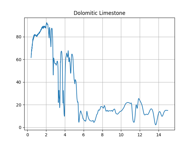
384|Dolomitic Limestone
Next, let’s retrieve and plot one of the results (we will take the last one).
In [6]: f = plt.figure()

In [7]: s = db.get_signature(384)

In [8]: import pylab as plt

In [9]: plt.plot(s.x, s.y)
Out[9]: [<matplotlib.lines.Line2D at 0x7f61aab7dcc0>]

In [10]: plt.title(s.sample_name)
Out[10]: Text(0.5, 1, 'Dolomitic Limestone')

In [11]: plt.grid(1)
See also
Module sqlite3
The sqlite3 module is included with Python 2.5+. Details on sqlite3
connectionandcursorobjects can be found in the Python sqlite3 documentation.
ENVI Spectral Libraries
While the EcostressDatabase provides a Python interface to the
ECOSTRESS Spectral Library, there may be times where you want to repeatedly access
a small, fixed subset of the spectra in the library and do not want to repeatedly
query the database. The ENVI file format enables storage of spectral libraries
(see ENVI Headers). SPy can read these files into a SPy
SpectralLibrary object.
To enable easy creation of custom spectral libraries, the EcostressDatabase
has a create_envi_spectral_library method that
generates a spectral library that can easily be saved to ENVI format. Spectra
in the ECOSTRESS library have varying numbers of samples over varying spectral
ranges. To generate the library we want to save to ENVI format, we need to specify
a band discretization to which we want all of the desired spectra resampled.
Let’s pick the bands from our sample hyperspectral image.
In [12]: bands = aviris.read_aviris_bands('92AV3C.spc')

In [13]: print(bands.centers[0], bands.centers[-1])
400.019989 2498.959961
We see from the output above that the bands range from about 400 - 2,500 nm (we’re ignoring the fact that the bands at both ends have a finite width). We would like to find library spectra that cover the entire spectral range for our image, so we’ll check the band limits for the library spectra. But first, let’s check the units of the spectra in the library.
In [14]: db.print_query('SELECT DISTINCT Measurement, XUnit, YUnit FROM Samples, Spectra ' +
   ....:                      'WHERE Samples.SampleID = Spectra.SampleID AND ' +
   ....:                      'Name LIKE "%stone%"')
   ....:
Hemispherical reflectance|Wavelength (micrometers)|Reflectance (percent)
Directional (10 Degree) Hemispherical Reflectance|Wavelength (micrometers)|Reflectance (percent)
Reflectance|Wavelength (micrometers)|Reflectance (percent)
Directional (10 degree) Hemispherical Reflectance|Wavelength (micrometers)|Reflectance (percent)
Directional (10 degree) hemispherical reflectance|Wavelength (micrometers)|Reflectance (percent)
Directional hemispherical reflectance|Wavelength (micrometers)|Reflectance (percent)
We see that all spectra are measures of reflectance but wavelengths are in units of micrometers, whereas our sample image bands are in nanometers. To properly query the spectra, we will need to specify the band limits in micrometers.
In [15]: db.print_query('SELECT COUNT() FROM Samples, Spectra ' +
   ....:       'WHERE Samples.SampleID = Spectra.SampleID AND ' +
   ....:       'Name LIKE "%stone%" AND ' +
   ....:       'MinWavelength <= 0.4 AND MaxWavelength >= 2.5')
   ....:
59
So it appears that 59 of the 78 “stone” spectra cover the desired band limits.
To create a new, resampled spectral library for these spectra, we call the
EcostressDatabase create_envi_spectral_library
method, passing it the list of spectrum IDs and our output band schema (in micrometers).
Since our bands are defined in nanometers, we will convert them before calling
the method.
In [16]: rows = db.query('SELECT SpectrumID FROM Samples, Spectra ' +
....: 'WHERE Samples.SampleID = Spectra.SampleID AND ' +
....: 'Name LIKE "%stone%" AND ' +
....: 'MinWavelength <= 0.4 AND MaxWavelength >= 2.5')
....:
In [17]: ids = [r[0] for r in rows]
In [18]: print(ids)
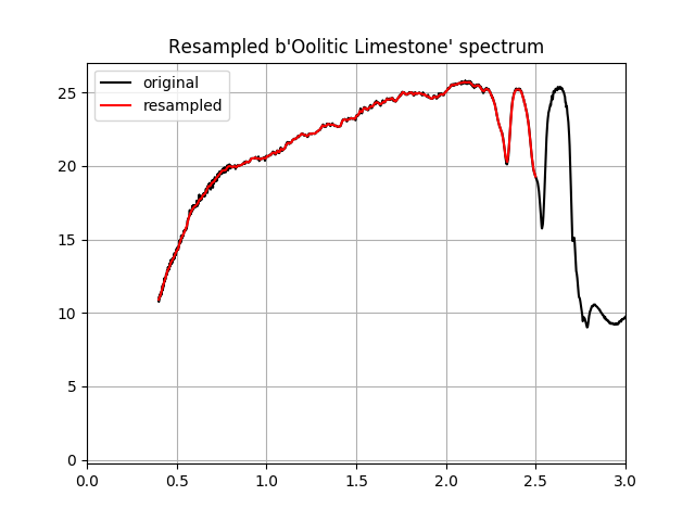
[14, 73, 167, 171, 203, 237, 275, 279, 384, 502, 532, 582, 601, 682, 744, 766, 788, 789, 1064, 1114, 1121, 1218, 1404, 1429, 1433, 1459, 1551, 1563, 1615, 1624, 1631, 1652, 1669, 1745, 1903, 1929, 2153, 2155, 2200, 2254, 2271, 2308, 2375, 2472, 2602, 2626, 2653, 2717, 2740, 2811, 2880, 3002, 3033, 3059, 3069, 3189, 3234, 3314, 3339]
In [19]: bands.centers = [x / 1000. for x in bands.centers]
In [20]: bands.bandwidths = [x / 1000. for x in bands.bandwidths]
In [21]: lib = db.create_envi_spectral_library(ids, bands)
Now that we’ve created a resampled library of spectra, let’s plot the last spectrum in the resampled library.
In [22]: f = plt.figure()

In [23]: s = db.get_signature(ids[-1])

In [24]: plt.plot(s.x, s.y, 'k-', label='original');

In [25]: plt.plot(bands.centers, lib.spectra[-1], 'r-', label='resampled');

In [26]: plt.grid(1)

In [27]: plt.gca().legend(loc='upper left');

In [28]: plt.xlim(0, 3);

In [29]: plt.title('Resampled %s spectrum' % lib.names[-1]);
The resampled spectral library can be used with any image that uses the same band calibration to which we resampled the spectra. We can also save the library for future use. But before we save the library, we need to change the band units to the units used in the band calibration (we need to convert from micrometers to nanometers).
In [30]: lib.bands.centers = [1000. * x for x in lib.bands.centers]

In [31]: lib.bands.bandwidths = [1000. * x for x in lib.bands.bandwidths]

In [32]: lib.bands.band_unit = 'nm'

In [33]: lib.save('stones', 'Stone spectra from the ECOSTRESS library')
Saving the library with the name “stones” creates two files: “stones.sli” and “stones.hdr”. The first file contains the resampled spectra and the second is the header file that we use to open the library.
In [34]: mylib = envi.open('stones.hdr')

In [35]: mylib
Out[35]: <spectral.io.envi.SpectralLibrary at 0x7f61aab7f7b8>
References
- Baldridge2009
Baldridge, A. M., Hook, S. J., Grove, C. I. and G. Rivera, 2008(9). The ASTER Spectral Library Version 2.0. In press Remote Sensing of Environment
- Meerdink2019
Meerdink, S. K., Hook, S. J., Roberts, D. A., & Abbott, E. A. (2019). The ECOSTRESS spectral library version 1.0. Remote Sensing of Environment, 230(111196), 1–8.